# load numpy as np, matplotlib as plt
%matplotlib inline
import numpy as np
import matplotlib.pyplot as pltNotebook 2: Model selection and evaluation
Notebook prepared by Chloé-Agathe Azencott with the help of Arthur Imbert and contributions from Giann Karlo.
The goals of this notebook will be:
- to evaluate a model on a test set.
- to choose the value of a hyperparameter of a learning algorithm.
- to understand the interest of polynomial regression and regularization.
plt.rc('font', **{'size': 12}) # sets the font size globally for the plots (in pt)import pandas as pd1. Loading data
Abalone
Determining the age of abalone based on physical measurements. The age of abalone is determined by cutting the shell across the cone, staining it, and counting the number of rings under a microscope—a laborious and time-consuming task. Other measurements, which are easier to obtain, are used to determine age. Our goal is therefore to predict the age of abalone automatically and help biologists determine the age of abalone in a given location.
Wine (optional)
We will work with a dataset containing physicochemical information on a number of Portuguese wines (vinho verde), as well as the ratings assigned to them by people who have tasted them. Our goal is to automate this process: we want to directly predict the rating of wines based on their physicochemical characteristics, in order to assist winemakers, improve wine production, and target the tastes of niche consumers.
Both datasets are available on the UCI Machine Learning Repository, where you’ll find many classic datasets: wine-quality and abalone. No need to download them; they’re already in your directory, in the file data/abalone.csv or data/winequality-white.csv. We’ll load them using pandas:
# df = pd.read_csv('data/abalone.csv', # nom du fichier
#                    sep="," # séparateur de colonnes
#                    )

# df = pd.read_csv('data/winequality-white.csv', # nom du fichier
#                    sep="," # séparateur de colonnes
#                    )
Alternatively: If you need to download the file (for example on colab):
#!wget https://raw.githubusercontent.com/chagaz/cp-ia-intro-ml-2022/main/2-Selection/data/winequality-white.csv
!wget https://raw.githubusercontent.com/ThomasWalter/CourseFoundationsML/SIA2025/Notebooks/2-Selection/data/abalone.csv

# df = pd.read_csv('winequality-white.csv', # nom du fichier
#                    sep=";" # séparateur de colonnes
#                    )

df = pd.read_csv('abalone.csv', # nom du fichier
                   sep="," # séparateur de colonnes
                   )
--2026-05-12 08:42:10-- https://raw.githubusercontent.com/ThomasWalter/CourseFoundationsML/SIA2025/Notebooks/2-Selection/data/abalone.csv
Resolving raw.githubusercontent.com (raw.githubusercontent.com)... 185.199.110.133, 185.199.108.133, 185.199.109.133, ...
Connecting to raw.githubusercontent.com (raw.githubusercontent.com)|185.199.110.133|:443... connected.
HTTP request sent, awaiting response... 200 OK
Length: 191962 (187K) [text/plain]
Saving to: ‘abalone.csv.4’
abalone.csv.4 0%[ ] 0 --.-KB/s
abalone.csv.4 100%[===================>] 187.46K --.-KB/s in 0.02s
2026-05-12 08:42:10 (7.50 MB/s) - ‘abalone.csv.4’ saved [191962/191962]
We can now examine this file directly in our notebook, for example by looking at the first lines:
df.head()| sex | length | diameter | height | whole-weight | shucked-weight | viscera-weight | shell-weight | rings | |
|---|---|---|---|---|---|---|---|---|---|
| 0 | M | 0.455 | 0.365 | 0.095 | 0.5140 | 0.2245 | 0.1010 | 0.150 | 15 |
| 1 | M | 0.350 | 0.265 | 0.090 | 0.2255 | 0.0995 | 0.0485 | 0.070 | 7 |
| 2 | F | 0.530 | 0.420 | 0.135 | 0.6770 | 0.2565 | 0.1415 | 0.210 | 9 |
| 3 | M | 0.440 | 0.365 | 0.125 | 0.5160 | 0.2155 | 0.1140 | 0.155 | 10 |
| 4 | I | 0.330 | 0.255 | 0.080 | 0.2050 | 0.0895 | 0.0395 | 0.055 | 7 |
Transformation one-hot
# Create a new dataframe where the 'sex' column is replaced with its one-hot encoding
df_dummies = pd.get_dummies(df, columns=['sex'])df_dummies.head()| length | diameter | height | whole-weight | shucked-weight | viscera-weight | shell-weight | rings | sex_F | sex_I | sex_M | |
|---|---|---|---|---|---|---|---|---|---|---|---|
| 0 | 0.455 | 0.365 | 0.095 | 0.5140 | 0.2245 | 0.1010 | 0.150 | 15 | False | False | True |
| 1 | 0.350 | 0.265 | 0.090 | 0.2255 | 0.0995 | 0.0485 | 0.070 | 7 | False | False | True |
| 2 | 0.530 | 0.420 | 0.135 | 0.6770 | 0.2565 | 0.1415 | 0.210 | 9 | True | False | False |
| 3 | 0.440 | 0.365 | 0.125 | 0.5160 | 0.2155 | 0.1140 | 0.155 | 10 | False | False | True |
| 4 | 0.330 | 0.255 | 0.080 | 0.2050 | 0.0895 | 0.0395 | 0.055 | 7 | False | True | False |
Creation of X and y data matrices
X = np.array(df_dummies.drop(columns=['rings']))y = np.array(df['rings'])print(X.shape, y.shape)(4177, 10) (4177,)Question: How many training examples are in the data? How many variables?
Transformation into a binary classification problem
We will try to classify the older and younger abalones (score >= 10).
y = np.where(y >= 10, 1, 0)Question: What do you think about using linear regression to solve this problem?
2. Separation of data into a training set and a test set
To be able to evaluate a learning model in an unbiased way, we need to create a test set containing data on which the model has not been trained. This test set corresponds to “new” data.
To do this, we will use the train_test_split function of the scikit-learn model_selection module:
from sklearn import model_selection

X_train, X_test, y_train, y_test = model_selection.train_test_split(X, y,
                                    test_size=0.3, # 30% of data in the test set
                                    random_state=42 # random generator seed
                                    )
Fixing the random generator seed allows us to get the same training and test sets by rerunning the command.
print(X_train.shape, X_test.shape, y_train.shape, y_test.shape)(2923, 10) (1254, 10) (2923,) (1254,)Question: How many samples does the training set (X_train, y_train) contain? And the test set (X_test, y_test)?
Transformation of variables
We saw in Notebook 1 that it is more reasonable to center-reduce the variables before proceeding.
Let’s not forget that the test set is supposedly unknown at the time of training: we must use only the training set to center-reduce the data.
from sklearn import preprocessing# Create a "standardizer" and calibrate it to the training data
std_scaler = preprocessing.StandardScaler().fit(X_train)
# Apply standardization to training data
X_train_scaled = std_scaler.transform(X_train)
# Apply standardization to test data
X_test_scaled = std_scaler.transform(X_test)3. Nearest neighbors
We will now evaluate the ability of a nearest neighbors algorithm to classify wines.
To do this, we use the KNeighborsClassifier class of the scikit-learn neighbors module.
from sklearn import neighborsTraining on the training set
As in Notebook 1, we start by instantiating an object of the class that interests us:
model_knn = neighbors.KNeighborsClassifier()We can then train it on the centered-reduced training data:
model_knn.fit(X_train_scaled, y_train)KNeighborsClassifier()In a Jupyter environment, please rerun this cell to show the HTML representation or trust the notebook.
On GitHub, the HTML representation is unable to render, please try loading this page with nbviewer.org.
KNeighborsClassifier()
Test set Predictions
We can now use the classifier trained on the test data, still centered-reduced:
y_pred_knn = model_knn.predict(X_test_scaled)Performance evaluation
Many metrics make it possible to evaluate the performance of a classification algorithm (see the scikit-learn doc on this subject). The confusion matrix in particular allows you to visualize how many examples of each class receive each label:
from sklearn import metricsmetrics.ConfusionMatrixDisplay.from_predictions(y_test, y_pred_knn)
NoteClick for figure
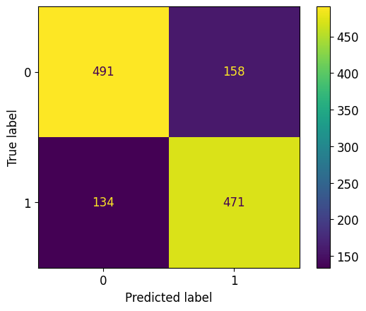
print(metrics.confusion_matrix(y_test, y_pred_knn))[[491 158]
[134 471]]Question: How many true positives are there? False negatives?
The confusion matrix can be summarized by the F1 score
F1 score is useful to evaluate the performance of a classification model. it combines two other important metrics: precision and recall. The F1 score is the harmonic mean of precision and recall, providing a single score that balances both.
The F1 score is valuable when you have an imbalanced dataset, for example, a dataset for misinformation where 99% of posts are not fake and only 1% are. A model that just predicts not fake every time would be 99% accurate, but it would be useless because it never finds the fake news. The F1 score provides a much better assessment in these cases.
print("F1 of kNN on the test set : %.3f" % metrics.f1_score(y_test, y_pred_knn))F1 of kNN on the test set : 0.7634. Selecting the number of nearest neighbors
Question: How many nearest neighbors were used in the previous section? Rely on the documentation, for example by typing:
help(neighbors.KNeighborsClassifier)In a cell below.
help(neighbors.KNeighborsClassifier)Setting up cross validation
The number of nearest neighbors (n_neighbors) is a hyperparameter of the nearest neighbors algorithm: it is not part of the parameters of the model learned by the algorithm, but we must set it ourselves before training.
We will now choose this number of nearest neighbors by a gridsearch procedure, which consists of comparing the performances of models trained using predefined values (the grid) of the hyperparameter.
Heads up ! If we want to be able to use the test set to evaluate the generalization error of the model using the optimal value of the number of nearest neighbors, we cannot use it also for this selection step, because otherwise we could bias the model and overlearn.
To compare our models on the training set, we will use cross-validation, once again thanks to the model-selection module from scikit-learn.
n_folds = 10

# Create a KFold object which will allow cross-validation in n_folds folds
kf = model_selection.KFold(n_splits=n_folds,
                           shuffle=True, # mix the samples before creating the folds
                           random_state=42
                          )

# Use kf to split the training set into n_folds folds.
# kf.split returns an iterator (consumed after a loop).
# To be able to use the same folds several times, we transform this iterator into a list of indices:
kf_indices = list(kf.split(X_train))
kf_indices contains 10 pairs of two index vectors.
Each of these pairs corresponds to a fold.
The first vector gives the indices of the samples forming the training part of this fold. The second gives the indices of the samples forming the test part of this fold.
for (idx, fold) in enumerate(kf_indices):
    print("The fold %d contains %d observations for training and %d observations for validation" % (idx, len(fold[0]), len(fold[1])))
The fold 0 contains 2630 observations for training and 293 observations for validation
The fold 1 contains 2630 observations for training and 293 observations for validation
The fold 2 contains 2630 observations for training and 293 observations for validation
The fold 3 contains 2631 observations for training and 292 observations for validation
The fold 4 contains 2631 observations for training and 292 observations for validation
The fold 5 contains 2631 observations for training and 292 observations for validation
The fold 6 contains 2631 observations for training and 292 observations for validation
The fold 7 contains 2631 observations for training and 292 observations for validation
The fold 8 contains 2631 observations for training and 292 observations for validation
The fold 9 contains 2631 observations for training and 292 observations for validationQuestion: How many times does each sample appear in the training portion of a fold? In the test part? (There is no need to write any code to answer.)
Grid search
k_values = np.arange(3, 50, step=2)k_valuesarray([ 3, 5, 7, 9, 11, 13, 15, 17, 19, 21, 23, 25, 27, 29, 31, 33, 35,
37, 39, 41, 43, 45, 47, 49])Question: Why select only odd numbers of neighbors?
We will now use the GridSearchCV class of the scikit-learn model_selection module to determine the optimal value of the number of nearest neighbors by grid search.
# Instantiating a GridSearchCV object
grid = model_selection.GridSearchCV(neighbors.KNeighborsClassifier(), # predictor to evaluate
                                    {'n_neighbors':k_values}, # hyperparameter value dictionary
                                    cv=kf_indices, # cross-validation to use
                                    scoring='f1' # performance evaluation metric
                                   )
We will also use the time magic command to measure the calculation time of a cell in our notebook.
%%time
# Using this object on training data (centered-reduced)
grid.fit(X_train_scaled, y_train)
CPU times: user 4.31 s, sys: 4.69 ms, total: 4.32 s
Wall time: 5.94 sGridSearchCV(cv=[(array([ 0, 1, 2, ..., 2919, 2920, 2922]),
array([ 30, 32, 44, 45, 51, 56, 63, 67, 70, 73, 80,
93, 102, 124, 141, 162, 175, 178, 194, 196, 203, 211,
239, 251, 256, 296, 298, 309, 318, 321, 322, 324, 331,
354, 368, 410, 411, 430, 433, 439, 460, 463, 471, 485,
486, 495, 506, 527, 528, 557, 564, 565, 568, 572, 581,
598, 599, 610, 642, 650, 662, 676, 677, 678, 679, 693,
700, 727, 729, 759, 785, 794, 802, 807, 811, 838...
2450, 2454, 2489, 2511, 2520, 2532, 2556, 2557, 2558, 2568, 2572,
2598, 2604, 2612, 2613, 2625, 2640, 2644, 2660, 2675, 2680, 2690,
2693, 2695, 2703, 2729, 2731, 2734, 2747, 2757, 2760, 2767, 2773,
2774, 2777, 2785, 2793, 2808, 2814, 2824, 2839, 2841, 2844, 2847,
2850, 2853, 2862, 2870, 2872, 2879]))],
estimator=KNeighborsClassifier(),
param_grid={'n_neighbors': array([ 3, 5, 7, 9, 11, 13, 15, 17, 19, 21, 23, 25, 27, 29, 31, 33, 35,
37, 39, 41, 43, 45, 47, 49])},
scoring='f1')In a Jupyter environment, please rerun this cell to show the HTML representation or trust the notebook. On GitHub, the HTML representation is unable to render, please try loading this page with nbviewer.org.
GridSearchCV(cv=[(array([   0,    1,    2, ..., 2919, 2920, 2922]),
                  array([  30,   32,   44,   45,   51,   56,   63,   67,   70,   73,   80,
         93,  102,  124,  141,  162,  175,  178,  194,  196,  203,  211,
        239,  251,  256,  296,  298,  309,  318,  321,  322,  324,  331,
        354,  368,  410,  411,  430,  433,  439,  460,  463,  471,  485,
        486,  495,  506,  527,  528,  557,  564,  565,  568,  572,  581,
        598,  599,  610,  642,  650,  662,  676,  677,  678,  679,  693,
        700,  727,  729,  759,  785,  794,  802,  807,  811,  838...
       2450, 2454, 2489, 2511, 2520, 2532, 2556, 2557, 2558, 2568, 2572,
       2598, 2604, 2612, 2613, 2625, 2640, 2644, 2660, 2675, 2680, 2690,
       2693, 2695, 2703, 2729, 2731, 2734, 2747, 2757, 2760, 2767, 2773,
       2774, 2777, 2785, 2793, 2808, 2814, 2824, 2839, 2841, 2844, 2847,
       2850, 2853, 2862, 2870, 2872, 2879]))],
             estimator=KNeighborsClassifier(),
             param_grid={'n_neighbors': array([ 3,  5,  7,  9, 11, 13, 15, 17, 19, 21, 23, 25, 27, 29, 31, 33, 35,
       37, 39, 41, 43, 45, 47, 49])},
scoring='f1')KNeighborsClassifier(n_neighbors=np.int64(23))
KNeighborsClassifier(n_neighbors=np.int64(23))
The optimal value of the hyperparameter is given by:
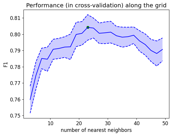
print(grid.best_params_){'n_neighbors': np.int64(23)}The following code displays the performance of the model according to the value of the hyperparameter:
mean_test_score = grid.cv_results_['mean_test_score']
stde_test_score = grid.cv_results_['std_test_score'] / np.sqrt(n_folds) # standard error

p = plt.plot(k_values, mean_test_score)
plt.plot(k_values, (mean_test_score + stde_test_score), '--', color=p[0].get_color())
plt.plot(k_values, (mean_test_score - stde_test_score), '--', color=p[0].get_color())
plt.fill_between(k_values, (mean_test_score + stde_test_score),
                 (mean_test_score - stde_test_score), alpha=0.2)

best_index = np.where(k_values == grid.best_params_['n_neighbors'])[0][0]
plt.scatter(k_values[best_index], mean_test_score[best_index])


plt.xlabel('number of nearest neighbors')
plt.ylabel('F1')
plt.title("Performance (in cross-validation) along the grid")
plt.show()
NoteClick for figure
Optimal nearest neighbor model
print("Best F1 in cross-validation: %.3f" % grid.best_score_)Best F1 in cross-validation: 0.804The model trained on the entire data provided to grid.fit with the best hyperparameter value(s) is given by grid.best_estimator_.
y_pred_knn_opt = grid.best_estimator_.predict(X_test_scaled)metrics.ConfusionMatrixDisplay.from_predictions(y_test, y_pred_knn_opt)
NoteClick for figure
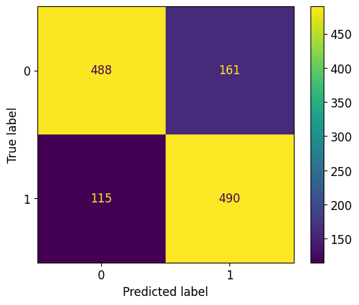
print("F1 of kNN (optimal k) on the test set : %.3f" % metrics.f1_score(y_test, y_pred_knn_opt))F1 of kNN (optimal k) on the test set : 0.7805. Regularized logistic regression
Performance of an unregularized logistic regression
We will now train a logistic regression (because we have a classification problem) on the training set and evaluate it on the test set.
We use the LogisticRegression class from the linear_model module of scikit-learn.
from sklearn import linear_model# Create a linear regression model
model_rlog = linear_model.LogisticRegression(penalty=None) # model not regularized for the moment
# Train this model on (X_train_scaled, y_train)
model_rlog.fit(X_train_scaled, y_train)LogisticRegression(penalty=None)In a Jupyter environment, please rerun this cell to show the HTML representation or trust the notebook.
On GitHub, the HTML representation is unable to render, please try loading this page with nbviewer.org.
LogisticRegression(penalty=None)
# Predict test set labels
y_pred_rlog = model_rlog.predict(X_test_scaled)
metrics.ConfusionMatrixDisplay.from_predictions(y_test, y_pred_rlog)
NoteClick for figure
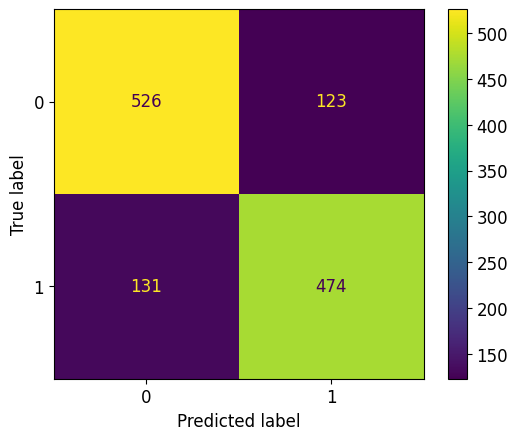
print("F1 score of a logistic regression on the test set: %.3f" % metrics.f1_score(y_test, y_pred_rlog))F1 score of a logistic regression on the test set: 0.789Question: What do you think of the quality of the model?
Model coefficients
# Calculate the number of variables
num_features = X_train.shape[1]

# Display for each variable its coefficient in the model
plt.scatter(range(num_features), # on the abscissa: indices of the variables
            model_rlog.coef_ # on the ordinate: their weight in the model
           )

# Label the x-axis tick marks
tmp = plt.xticks(range(num_features), # one mark per variable
                 list(df_dummies.drop(columns=['rings']).columns),  # display variable name
                 rotation=90, # turn labels 90 degrees
                 fontsize=14)

# Label the axes
tmp = plt.xlabel('Variable', fontsize=14)
tmp = plt.ylabel('Coefficient', fontsize=14)
plt.show()
NoteClick for figure
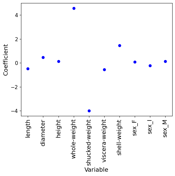
# Display the coefficients with their corresponding variable names
for i, col_name in enumerate(df_dummies.drop(columns=['rings']).columns):
    print(f"{col_name}: {model_rlog.coef_[0][i]:.4f}")
length: -0.4844
diameter: 0.4712
height: 0.1382
whole-weight: 4.5643
shucked-weight: -3.9831
viscera-weight: -0.5650
shell-weight: 1.4623
sex_F: 0.0886
sex_I: -0.2200
sex_M: 0.1267Ridge regularization
We will now add an l2 (or ridge) regularization to this logistic regression.
Here there are few variables and their coefficients take low values: it is not certain that regularization is necessary, but as this dataset has few variables, we can use it to look at the effect of regularization on the values of the coefficients of the learned model.
Let’s start by giving ourselves a grid of values for the regularization parameter C.
Watch out! The larger C is, the less there is regularization.
c_values = np.logspace(-6, 6, 50)
c_values
array([1.00000000e-06, 1.75751062e-06, 3.08884360e-06, 5.42867544e-06,
9.54095476e-06, 1.67683294e-05, 2.94705170e-05, 5.17947468e-05,
9.10298178e-05, 1.59985872e-04, 2.81176870e-04, 4.94171336e-04,
8.68511374e-04, 1.52641797e-03, 2.68269580e-03, 4.71486636e-03,
8.28642773e-03, 1.45634848e-02, 2.55954792e-02, 4.49843267e-02,
7.90604321e-02, 1.38949549e-01, 2.44205309e-01, 4.29193426e-01,
7.54312006e-01, 1.32571137e+00, 2.32995181e+00, 4.09491506e+00,
7.19685673e+00, 1.26485522e+01, 2.22299648e+01, 3.90693994e+01,
6.86648845e+01, 1.20679264e+02, 2.12095089e+02, 3.72759372e+02,
6.55128557e+02, 1.15139540e+03, 2.02358965e+03, 3.55648031e+03,
6.25055193e+03, 1.09854114e+04, 1.93069773e+04, 3.39322177e+04,
5.96362332e+04, 1.04811313e+05, 1.84206997e+05, 3.23745754e+05,
5.68986603e+05, 1.00000000e+06])We will now not use GridSearchCV but implement our grid search ourselves, in order to have access to the values of the coefficients of each of the models:
%%time
f1_per_c = [] # to record the F1 score values for each of the 50 values of C
weights_per_c = [] # to record the coefficients associated with each variable,
# for the 50 values of C
for c_val in c_values:
# Create a logistic regression model regularized by the c_val parameter
model_ridge = linear_model.LogisticRegression(penalty='l2', C=c_val)
# Calculate the cross-validation performance of the model
f1 = model_selection.cross_val_score(model_ridge, # predictor to evaluate
X_train_scaled, y_train, # training data
cv=kf_indices, # cross-validation to use
scoring='f1' # performance evaluation metric
)
f1_per_c.append(f1)
# Train the model on the total training set
model_ridge.fit(X_train_scaled, y_train)
# Save regression coefficients
weights_per_c.append(model_ridge.coef_[0])CPU times: user 18.3 s, sys: 39.3 ms, total: 18.4 s
Wall time: 10.8 sEvolution of performance according to the regularization coefficient
mean_test_score = np.mean(np.array(f1_per_c), axis=1)
stde_test_score = np.std(np.array(f1_per_c), axis=1) / np.sqrt(n_folds) # standard error

p = plt.plot(c_values, mean_test_score)
plt.plot(c_values, (mean_test_score + stde_test_score), '--',
         color=p[0].get_color()) # reuse the same color as before instead of moving forward
plt.plot(c_values, (mean_test_score - stde_test_score), '--', color=p[0].get_color())
plt.fill_between(c_values, (mean_test_score + stde_test_score),
                 (mean_test_score - stde_test_score), alpha=0.2)


plt.xscale('log') # use a logarithmic abscissa scale

# Label the axes
tmp = plt.xlabel('Value of C', fontsize=14)
tmp = plt.ylabel('Average F1', fontsize=14)

# Title
tmp = plt.title("Performance (cross-validation) of logistic regression", fontsize=14)
NoteClick for figure
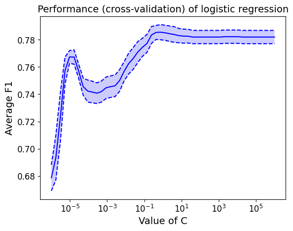
Question: How does the model error (in cross-validation) scale with the amount of regularization?
Optimal ridge regression model
# Find the index of the optimal value of C
best_C_idx = np.argmax(np.mean(f1_per_c, axis=1))

# Optimal C value
c_opt = c_values[best_C_idx]
print("Optimal C value (ridge regression): %.3e" % c_opt)

# Corresponding MSE
print("F1 score (cross-validation) of the optimal regularized logistic regression model: %.2f +/- %.2f" %  \
      (np.mean(np.array(f1_per_c)[best_C_idx]), # average value
      np.std(np.array(f1_per_c)[best_C_idx]) # standard deviation
     ))
Optimal C value (ridge regression): 7.543e-01
F1 score (cross-validation) of the optimal regularized logistic regression model: 0.79 +/- 0.02Evolution of regression coefficients as a function of regularization
# Create a figure
fig = plt.figure(figsize=(8, 5))
# Changing colors for better visualization
plt.rcParams['axes.prop_cycle'] = plt.cycler(color=['blue', 'green', 'red', 'cyan', 'magenta', 'yellow', 'black', 'purple', 'pink', 'brown', 'orange', 'teal', 'coral', 'lightblue', 'lime', 'lavender', 'turquoise', 'darkgreen', 'tan', 'salmon', 'gold'])
lines = plt.plot(c_values,
weights_per_c # ordinate = values of regression coefficients
)
plt.xscale('log') # logarithmic scale in abscissa
# Display again (at the abscissa 2x1e6) the regression coefficients obtained without regularization
for coeff in model_rlog.coef_[0]:
plt.scatter([2e6], [coeff])
# Mark the optimal value of C with a vertical bar
plt.plot([c_opt, c_opt], [-5, 5], 'k--')
# Show legend
tmp = plt.legend(lines, # retrieve the identifier
list(df.columns), # name of each variable, excluding 'quality'
frameon=False, # no frame around the legend
loc=(1, 0), # place the caption to the right of the image
fontsize=14)
tmp = plt.xlabel('Value of C', fontsize=14)
tmp = plt.ylabel('Regression coefficient', fontsize=14)
tmp = plt.title('Logistic regression', fontsize=16)
plt.show()
NoteClick for figure
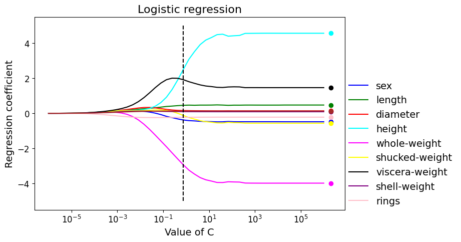
# Get the coefficients of the best estimator from the grid search
optimal_coefficients = weights_per_c[best_C_idx]

# Display the coefficients with their corresponding variable names
for i, col_name in enumerate(df_dummies.drop(columns=['rings']).columns):
    print(f"{col_name}: {optimal_coefficients[i]:.4f} ")
length: -0.3808
diameter: 0.4567
height: 0.1565
whole-weight: 2.5060
shucked-weight: -2.9410
viscera-weight: -0.1223
shell-weight: 1.9154
sex_F: 0.0951
sex_I: -0.2285
sex_M: 0.1285 Question: How do the model coefficients change depending on the amount of regularization?
Question: Do these coefficients seem consistent with those obtained for non-regularized logistic regression?
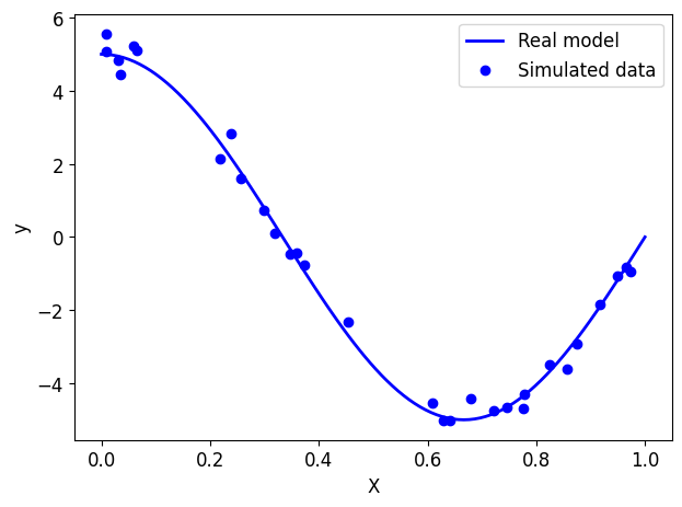
6. Ridge regularization on a textbook case
To better understand ridge regularization, we will simulate a non-linear data set which will take the form of a sinusoidal curve.
Data simulation
nb_samples = 30

np.random.seed(13)

# real model
def true_model(X):
    return np.cos(1.5 * np.pi * X) * 5

# "ground truth" samples taken from the real model
X_ground_truth = np.linspace(0, 1, 100).reshape(-1, 1)
y_ground_truth = true_model(X_ground_truth)

# data = observations taken from the real model then noisy
X = np.sort(np.random.rand(nb_samples, 1))
y = true_model(X)
# adding noise
y += np.random.randn(nb_samples, 1) * 0.3

print(X.shape, y.shape)
(30, 1) (30, 1)# Draw the real model
plt.plot(X_ground_truth, y_ground_truth, label="Real model", linewidth=2)
# View simulated data
plt.scatter(X, y, label="Simulated data", marker="o")
plt.xlabel("X")
plt.ylabel("y")
plt.legend(loc="best")
plt.tight_layout()
plt.show()
NoteClick for figure
Training/test split
X_train, X_test, y_train, y_test = model_selection.train_test_split(X, y, test_size=0.3)
print(X_train.shape, y_train.shape)
print(X_test.shape, y_test.shape)
(21, 1) (21, 1)
(9, 1) (9, 1)Linear regression
Question: How many variables do we have in our problem?
Let’s train a “classic” linear regression (like the one seen in Notebook 1) on (X_train, y_train) and evaluate its performance on the training set and on the test set.
Question: Why compare these two performances?
# Training - initialize linear regression
reg = linear_model.LinearRegression()
# Train the linear model
reg.fit(X_train, y_train)LinearRegression()In a Jupyter environment, please rerun this cell to show the HTML representation or trust the notebook.
On GitHub, the HTML representation is unable to render, please try loading this page with nbviewer.org.
LinearRegression()
Performance
# RMSE
print("RMSE of a linear regression:")
# On the training set
rmse_reg_train = metrics.root_mean_squared_error(y_train, reg.predict(X_train))
print("\r train: {0:0.2f}".format(rmse_reg_train))
# On the test set
rmse_reg_test = metrics.root_mean_squared_error(y_test, reg.predict(X_test))
print("\r test: {0:0.2f}".format(rmse_reg_test))
RMSE of a linear regression:
train: 2.08
test: 1.91We will now display the model learned on the previous graph.
# Draw the real model
plt.plot(X_ground_truth, y_ground_truth, label="Real model", linewidth=2)

# Show learned model
y_model = reg.predict(X_ground_truth)
plt.plot(X_ground_truth, y_model, label="Model learned", linewidth=2)

# View simulated data
plt.scatter(X_train, y_train, label="Simulated data (train)", marker="o")
plt.scatter(X_test, y_test, label="Simulated data (test)", marker="D")

# plot format
plt.xlabel("X")
plt.ylabel("y")
plt.title("Linear regression")
plt.legend(loc="best")
plt.tight_layout()
plt.show()
NoteClick for figure
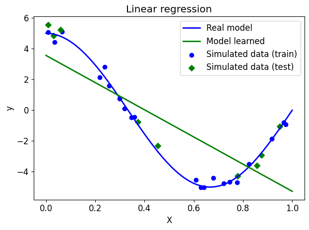
Question: What do you think of the performance of linear regression here?
Polynomial regression
Polynomial regression consists of learning a non-linear model by learning a linear model on a new set of variables, formed from mononoms of the variables describing our data.
Generally speaking, for a problem described by \(p\) variables \((X_1, X_2, \dots, X_p)\), a polynomial regression of degree \(d\) is a linear regression on the variables \((X_1, X_2, \dots, X_p, X_1^2, X_2^2 X_3^2, \dots, X_p^2, \dots, X_p^d)\). Note that we are thus creating a large number of variables that are correlated with each other; we gain in modeling finesse, but lose in model complexity, risk of overfitting, and the curse of dimensionality.
Such a transformation is possible with the PolynomialFeatures class of sklearn.preprocessing.
Here, we are regressing a line based on the powers of \(X\) rather than \(X\) alone: we are approximating the true model using a polynomial.
# calculation of powers of x, up to degree 15
polynomial_features = preprocessing.PolynomialFeatures(degree=15)# , include_bias=False)

# creation of corresponding datasets
X_train_poly = polynomial_features.fit_transform(X_train)
X_test_poly = polynomial_features.transform(X_test)
X_ground_truth_poly = polynomial_features.transform(X_ground_truth)

print(X_train_poly.shape)
print(X_test_poly.shape)
print(X_ground_truth_poly.shape)
(21, 16)
(9, 16)
(100, 16)Question: How many variables do we have now?
# Training
reg_poly = linear_model.LinearRegression()
reg_poly.fit(X_train_poly, y_train)LinearRegression()In a Jupyter environment, please rerun this cell to show the HTML representation or trust the notebook.
On GitHub, the HTML representation is unable to render, please try loading this page with nbviewer.org.
LinearRegression()
Performance
# RMSE
print("RMSE of a polynomial regression:")
# On the training set
rmse_reg_poly_train = metrics.root_mean_squared_error(y_train, reg_poly.predict(X_train_poly))
print("\r train: {0:0.2f}".format(rmse_reg_poly_train))
# On the test set
rmse_reg_poly_test = metrics.root_mean_squared_error(y_test, reg_poly.predict(X_test_poly))
print("\r test: {0:0.2f}".format(rmse_reg_poly_test))
RMSE of a polynomial regression:
train: 0.17
test: 1.10Question: Compare the performance of the model on the training set and the test set. What to conclude?
We will now display the model learned on the previous graph.
# Draw the real model
plt.plot(X_ground_truth, y_ground_truth, label="Real model", linewidth=2)

# Show learned model
plt.plot(X_ground_truth, reg_poly.predict(X_ground_truth_poly), label="Model learned", linewidth=2)

# View simulated data
plt.scatter(X_train, y_train, label="Simulated data (train)", marker="o")
plt.scatter(X_test, y_test, label="Simulated data (test)", marker="D")

# plot format
plt.xlabel("X")
plt.ylabel("y")
plt.title("Polynomial regression")
plt.legend(loc="best")
plt.tight_layout()
plt.ylim([-6, 6])
plt.show()
NoteClick for figure
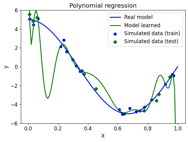
Question: What can you conclude about choosing polynomial regression?
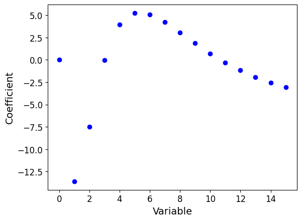
Model coefficients
# Calculate the number of variables
num_features = X_train_poly.shape[1]

# Display for each variable its coefficient in the model
plt.scatter(range(num_features), # on the abscissa: indices of the variables
            reg_poly.coef_ # on the ordinate: their weight in the model
           )

# Label the axes
tmp = plt.xlabel('Variable', fontsize=14)
tmp = plt.ylabel('Coefficient', fontsize=14)
plt.yscale("log")
NoteClick for figure
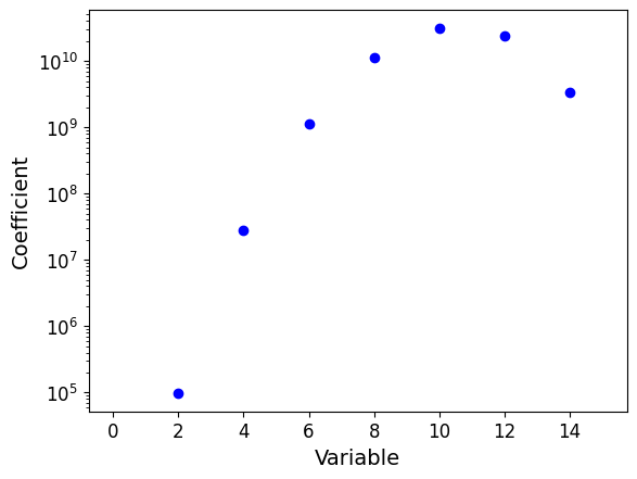
Question: What do you notice? Pay close attention to the scale of the coefficients.
Ridge regularized polynomial regression
As polynomial regression overfits, we will now apply a ridge regularization term to it to try to compensate for this effect.
# Training
ridge_poly = linear_model.Ridge(alpha=0.01, random_state=13)
ridge_poly.fit(X_train_poly, y_train)
Ridge(alpha=0.01, random_state=13)In a Jupyter environment, please rerun this cell to show the HTML representation or trust the notebook.
On GitHub, the HTML representation is unable to render, please try loading this page with nbviewer.org.
Ridge(alpha=0.01, random_state=13)
Performance
# RMSE
print("RMSE of a regularized polynomial regression:")
# On the training set
rmse_ridge_poly_train = metrics.root_mean_squared_error(y_train, ridge_poly.predict(X_train_poly))
print("\r train: {0:0.2f}".format(rmse_ridge_poly_train))
# On the test set
rmse_ridge_poly_test = metrics.root_mean_squared_error(y_test, ridge_poly.predict(X_test_poly))
print("\r test: {0:0.2f}".format(rmse_ridge_poly_test))
RMSE of a regularized polynomial regression:
train: 0.38
test: 0.30Question: Compare the performance of the model on the training set and the test set. What to conclude?
We will now display the model learned on the previous graph.
# Draw the real model
plt.plot(X_ground_truth, y_ground_truth, label="Real model", linewidth=2)

# Show learned model
plt.plot(X_ground_truth, ridge_poly.predict(X_ground_truth_poly), label="Model learned", linewidth=2)

# View simulated data
plt.scatter(X_train, y_train, label="Simulated data (train)", marker="o")
plt.scatter(X_test, y_test, label="Simulated data (test)", marker="D")

# plot format
plt.xlabel("X")
plt.ylabel("y")
plt.title("Regularized polynomial regression")
plt.legend(loc="best")
plt.tight_layout()
plt.show()
NoteClick for figure
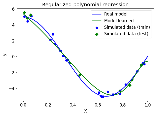
Question: What can you conclude about choosing Ridge regularization?
Model coefficients
# Calculate the number of variables
num_features = X_train_poly.shape[1]

# Display for each variable its coefficient in the model
plt.scatter(range(num_features), # on the abscissa: indices of the variables
            ridge_poly.coef_ # on the ordinate: their weight in the model
           )

# Label the axes
tmp = plt.xlabel('Variable', fontsize=14)
tmp = plt.ylabel('Coefficient', fontsize=14)
NoteClick for figure
Question: What do you notice now? What is the effect of regularization on the model coefficients?
Lasso regularized polynomial regression
# Training
lasso_poly = linear_model.Lasso(alpha=0.01, random_state=13)
lasso_poly.fit(X_train_poly, y_train)
Lasso(alpha=0.01, random_state=13)In a Jupyter environment, please rerun this cell to show the HTML representation or trust the notebook.
On GitHub, the HTML representation is unable to render, please try loading this page with nbviewer.org.
Lasso(alpha=0.01, random_state=13)
Performance
# RMSE
print("RMSE of a regularized polynomial regression:")
# On the training set
rmse_lasso_poly_train = metrics.root_mean_squared_error(y_train, lasso_poly.predict(X_train_poly))
print("\r train: {0:0.2f}".format(rmse_lasso_poly_train))
# On the test set
rmse_lasso_poly_test = metrics.root_mean_squared_error(y_test, lasso_poly.predict(X_test_poly))
print("\r test: {0:0.2f}".format(rmse_lasso_poly_test))
RMSE of a regularized polynomial regression:
train: 0.52
test: 0.41We will now display the model learned on the previous graph.
# Draw the real model
plt.plot(X_ground_truth, y_ground_truth, label="Real model", linewidth=2)

# Show learned model
plt.plot(X_ground_truth, lasso_poly.predict(X_ground_truth_poly), label="Model learned", linewidth=2)

# View simulated data
plt.scatter(X_train, y_train, label="Simulated data (train)", marker="o")
plt.scatter(X_test, y_test, label="Simulated data (test)", marker="D")

# plot format
plt.xlabel("X")
plt.ylabel("y")
plt.title("l1 regularized polynomial regression")
plt.legend(loc="best")
plt.tight_layout()
plt.show()
NoteClick for figure

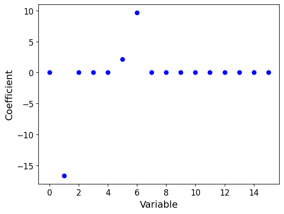
Model coefficients
# Calculate the number of variables
num_features = X_train_poly.shape[1]

# Display for each variable its coefficient in the model
plt.scatter(range(num_features), # on the abscissa: indices of the variables
            lasso_poly.coef_ # on the ordinate: their weight in the model
           )

# Label the axes
tmp = plt.xlabel('Variable', fontsize=14)
tmp = plt.ylabel('Coefficient', fontsize=14)
NoteClick for figure
Conclusion
We reached the end of this notebook. Here is a summary of what we have covered, with the key takeaways:
- We used the
scikit-learnlibrary to classify the age of abalone (or the quality of wine) based on continuous variables (characteristics of the abalone or wine). - We tried a first classifier model: KNeighborsClassifier (after data scaling).
- We evaluated the model perfomance based on a confusion matrix, and using the F1 score, which balances both precision and recall.
- We used cross-validation and grid search to find the best F1 score by testing a range of numbers representing neighbors. Cross-validation allows to assess how well a model generalizes to unseen data by splitting the dataset into multiple subsets. Grid search enables hyperparameter optimization by systematically testing combinations or range of different values for hyperparameters, such as the number of neighbors.
We manually performed a grid search on the effects of regularization by testing the hyperparameter C, remember, the larger C is, the less the is regularization. Finally, we explored ridge regularization on polynomial regression. We saw how a polynomial function of degree 15 can overfit the ground truth, but after applying a reguarization technique (ridge or lasso), there is a better fit.