Notebook 4 : Trees and Ensemble Methods

Notebook prepared by Chloé-Agathe Azencott and contributions from Giann Karlo.

In this notebook, we will discover decision trees and ensemble methods (random forests, gradient boosting).

# load numpy as np, matplotlib as plt
%matplotlib inline
import numpy as np
import matplotlib.pyplot as plt

plt.rc('font', **{'size': 12}) # sets the global font size for plots (in pt)

import pandas as pd

1. Data Loading

The goal of this notebook is to use the visual description of a mushroom to predict whether it is edible or not.

The data is available in data/mushrooms.csv. It comes from the dataset https://archive.ics.uci.edu/ml/datasets/Mushroom but slightly modified.

It contains a first line (header) describing the columns, then one line per mushroom. The values of the different variables are all represented by letters; here is their meaning:

cap-shape: bell=b,conical=c,convex=x,flat=f, knobbed=k,sunken=s
cap-surface: fibrous=f,grooves=g,scaly=y,smooth=s
cap-color: brown=n,buff=b,cinnamon=c,gray=g,green=r, pink=p,purple=u,red=e,white=w,yellow=y
bruises: bruises=t,no=f
odor: almond=a,anise=l,creosote=c,fishy=y,foul=f, musty=m,none=n,pungent=p,spicy=s
gill-attachment: attached=a,descending=d,free=f,notched=n
gill-spacing: close=c,crowded=w,distant=d
gill-size: broad=b,narrow=n
gill-color: black=k,brown=n,buff=b,chocolate=h,gray=g, green=r,orange=o,pink=p,purple=u,red=e, white=w,yellow=y
stalk-shape: enlarging=e,tapering=t
stalk-root: bulbous=b,club=c,cup=u,equal=e, rhizomorphs=z,rooted=r,missing=?
stalk-surface-above-ring: fibrous=f,scaly=y,silky=k,smooth=s
stalk-surface-below-ring: fibrous=f,scaly=y,silky=k,smooth=s
stalk-color-above-ring: brown=n,buff=b,cinnamon=c,gray=g,orange=o, pink=p,red=e,white=w,yellow=y
stalk-color-below-ring: brown=n,buff=b,cinnamon=c,gray=g,orange=o, pink=p,red=e,white=w,yellow=y
veil-type: partial=p,universal=u
veil-color: brown=n,orange=o,white=w,yellow=y
ring-number: none=n,one=o,two=t
ring-type: cobwebby=c,evanescent=e,flaring=f,large=l, none=n,pendant=p,sheathing=s,zone=z
spore-print-color: black=k,brown=n,buff=b,chocolate=h,green=r, orange=o,purple=u,white=w,yellow=y
population: abundant=a,clustered=c,numerous=n, scattered=s,several=v,solitary=y
habitat: grasses=g,leaves=l,meadows=m,paths=p, urban=u,waste=w,woods=d

The first column tells us the class of each mushroom, ‘e’ for edible and ‘p’ for poisonous.

Alternatively: If you need to download the file (e.g., on Colab), uncomment the following two lines:

# !wget https://raw.githubusercontent.com/CBIO-mines/fml-dassault-systems/main/data/mushrooms.csv

# df = pd.read_csv("mushrooms.csv")
df = pd.read_csv("https://raw.githubusercontent.com/CBIO-mines/fml-dassault-systems/main/data/mushrooms.csv")

# df = pd.read_csv('data/mushrooms.csv')
df.shape

(8124, 23)

df.head()

	class	cap-shape	cap-surface	cap-color	bruises	odor	gill-attachment	gill-spacing	gill-size	gill-color	...	stalk-surface-below-ring	stalk-color-above-ring	stalk-color-below-ring	veil-type	veil-color	ring-number	ring-type	spore-print-color	population	habitat
0	p	x	s	n	t	p	f	c	n	k	...	s	w	w	p	w	o	p	k	s	u
1	e	x	s	y	t	a	f	c	b	k	...	s	w	w	p	w	o	p	n	n	g
2	e	b	s	w	t	l	f	c	b	n	...	s	w	w	p	w	o	p	n	n	m
3	p	x	y	w	t	p	f	c	n	n	...	s	w	w	p	w	o	p	k	s	u
4	e	x	s	g	f	n	f	w	b	k	...	s	w	w	p	w	o	e	n	a	g

5 rows × 23 columns

Converting variables to numerical values

Our variables are currently categorical.

For example, for the “cap shape” variable, b corresponds to a bell cap, c to a conical cap, f to a flat cap, k to a knobbed cap, s to a sunken cap, and x to a convex cap.

To work with this data, we need to convert these categories into numerical values.

One possibility is to convert each letter into a number between 0 and the total number of categories, using preprocessing.LabelEncoder.

This encoding is not necessarily ideal: an algorithm that uses Euclidean distance will consider a convex cap (x converted to 5) to be closer to a sunken cap (s converted to 4) than to a conical cap (c converted to 1), which doesn’t make much sense. However, this is not a problem for algorithms based on decision trees, which treat categories as such and not as numerical values. The conversion is only necessary for implementation reasons.

One-hot encoding is generally a better choice. Note, however, that it has the disadvantage of increasing the number of variables and creating correlated variables.

from sklearn import preprocessing

label_encoder = preprocessing.LabelEncoder()

# manual_class = {'e': 1, 'p': 0}
# df['class'] = df['class'].map(manual_class)

for col in df.columns[:]:
    df[col] = label_encoder.fit_transform(df[col])

We can observe our data again:

df.head()

	class	cap-shape	cap-surface	cap-color	bruises	odor	gill-attachment	gill-spacing	gill-size	gill-color	...	stalk-surface-below-ring	stalk-color-above-ring	stalk-color-below-ring	veil-color	ring-number	ring-type	spore-print-color	population	habitat
0	1	5	2	4	1	6	1	0	1	4	...	2	7	7	2	1	4	2	3	5
1	0	5	2	9	1	0	1	0	0	4	...	2	7	7	2	1	4	3	2	1
2	0	0	2	8	1	3	1	0	0	5	...	2	7	7	2	1	4	3	2	3
3	1	5	3	8	1	6	1	0	1	5	...	2	7	7	2	1	4	2	3	5
4	0	5	2	3	0	5	1	1	0	4	...	2	7	7	2	1	0	3	0	1

5 rows × 23 columns

Creating the X and y data matrices

X = np.array(df.drop(columns=['class']))
y = np.array(df['class'])
print(X.shape, y.shape)

(8124, 22) (8124,)

Question: How many samples (examples) does our dataset contain? How many variables?

Click for answer

Our dataset contains 8124 samples (examples) and 22 variables (features) in X, and the target variable y has 8124 samples.

2. Selection and evaluation framework

We can now split our data into a training set and a test set, and then fix a split of the training set into 10 folds for cross-validation.

You will need the functions train_test_split and KFold

from sklearn import model_selection

Training and test set

### START OF YOUR CODE
X_train, X_test, y_train, y_test = model_selection.train_test_split(X, y, test_size=0.25, random_state=42)
### END OF YOUR CODE

Cross-validation

n_folds = 10

### START OF YOUR CODE

# Create a KFold object that will allow cross-validation in n_folds folds
kf = model_selection.KFold(n_splits=n_folds, shuffle=True, random_state=42)

# Use kf to split the training set into n_folds folds.
# kf.split returns an iterator (consumed after a loop).
# To use the same folds multiple times, we convert this iterator into a list of indices:
kf_indices = list(kf.split(X_train))

### END OF YOUR CODE

3. Decision Tree

We will now use a decision tree to learn a classifier on our data.

Decision trees are implemented in the DecisionTreeClassifier class of scikit-learn’s tree module.

from sklearn import tree

Decision tree with default hyperparameters

Let’s determine the F1 score using cross-validation for a decision tree with default hyperparameters in scikit-learn:

model_tree_default = tree.DecisionTreeClassifier()

f1_tree_default = model_selection.cross_val_score(model_tree_default, # predictor to evaluate
                                                  X_train, y_train, # training data
                                                  cv=kf_indices, # cross-validation to use
                                                  scoring='f1' # performance evaluation metric
                                                  )
print("F1 of a decision tree (default) in cross-validation: %.3f +/- %.3f" % (np.mean(f1_tree_default), np.std(f1_tree_default)))

F1 of a decision tree (default) in cross-validation: 0.878 +/- 0.016

Question: What do you think of this performance?

Click for answer

The default Decision Tree achieved an F1 score of approximately 0.878 +/- 0.014 in cross-validation. This indicates a reasonably good performance, but there might be room for improvement by optimizing its hyperparameters, especially its depth, to prevent overfitting or underfitting.

Cross-validation of decision tree depth

By default (see the documentation), we used a decision tree with maximum depth. We will now consider the tree depth (max_depth) as a hyperparameter to optimize using a grid search. We are re-using and adapting the code used for kNN in Notebook 3.

Let’s start by defining the grid:

d_values = np.arange(2, 31)

d_values

array([ 2,  3,  4,  5,  6,  7,  8,  9, 10, 11, 12, 13, 14, 15, 16, 17, 18,
       19, 20, 21, 22, 23, 24, 25, 26, 27, 28, 29, 30])

We can now use GridSearchCV:

# Instantiation of a GridSearchCV object
grid_tree = model_selection.GridSearchCV(tree.DecisionTreeClassifier(), # predictor to evaluate
                                         {'max_depth': d_values}, # dictionary of hyperparameter values
                                         cv=kf_indices, # cross-validation to use
                                         scoring='f1' # performance evaluation metric
                                         )

%%time

# Use this object on the training data
grid_tree.fit(X_train, y_train)

CPU times: user 3.81 s, sys: 4.01 ms, total: 3.82 s
Wall time: 3.82 s

GridSearchCV(cv=[(array([   0,    1,    2, ..., 6090, 6091, 6092], shape=(5483,)),
                  array([   8,   14,   15,   17,   23,   31,   33,   37,   44,   50,   65,
         79,   80,   84,   88,   93,  101,  132,  156,  157,  167,  168,
        177,  181,  185,  198,  199,  221,  228,  230,  233,  239,  254,
        259,  263,  279,  296,  308,  319,  323,  324,  325,  346,  351,
        371,  373,  393,  401,  408,  410,  420,  426,  439,  465,  469,
        472,  476,  491,  501,  506,  530,  534,  535,  538,  544,  549,
        553,  561,  565,  576,  586,  599,  604,  62...
       5791, 5794, 5814, 5815, 5820, 5847, 5848, 5855, 5862, 5864, 5865,
       5878, 5886, 5892, 5915, 5924, 5944, 5949, 5959, 5960, 5975, 5989,
       6007, 6012, 6014, 6021, 6029, 6031, 6032, 6035, 6036, 6069, 6070,
       6072, 6079, 6081, 6084]))],
             estimator=DecisionTreeClassifier(),
             param_grid={'max_depth': array([ 2,  3,  4,  5,  6,  7,  8,  9, 10, 11, 12, 13, 14, 15, 16, 17, 18,
       19, 20, 21, 22, 23, 24, 25, 26, 27, 28, 29, 30])},
             scoring='f1')

In a Jupyter environment, please rerun this cell to show the HTML representation or trust the notebook.
On GitHub, the HTML representation is unable to render, please try loading this page with nbviewer.org.

The optimal hyperparameter value is given by:

print(grid_tree.best_params_)

{'max_depth': np.int64(6)}

The following code allows displaying the model’s performance according to the hyperparameter value:

mean_test_score = grid_tree.cv_results_['mean_test_score']
stde_test_score = grid_tree.cv_results_['std_test_score'] / np.sqrt(n_folds) # standard error

plt.plot(d_values, mean_test_score)
plt.plot(d_values, (mean_test_score + stde_test_score), '--', color='steelblue')
plt.plot(d_values, (mean_test_score - stde_test_score), '--', color='steelblue')
plt.fill_between(d_values, (mean_test_score + stde_test_score),
                 (mean_test_score - stde_test_score), alpha=0.2)

best_index = np.where(d_values == grid_tree.best_params_['max_depth'])[0][0]
plt.scatter(d_values[best_index], mean_test_score[best_index])


plt.xlabel('maximum depth')
plt.ylabel('F1')
plt.title("Performance (in cross-validation) along the grid")

Text(0.5, 1.0, 'Performance (in cross-validation) along the grid')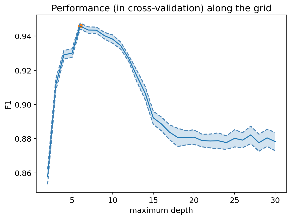

Question: What do you think of this performance?

Click for answer

The cross-validation results show that optimizing the max_depth hyperparameter significantly improves the Decision Tree’s performance. The optimal max_depth is 6, which yields a best F1 score of approximately 0.94. This is a substantial improvement over the default Decision Tree’s F1 score of 0.878. The plot illustrates that performance generally increases with depth up to a certain point, after which it plateaus or slightly decreases, indicating a good balance between bias and variance is achieved at max_depth=6.

Optimal decision tree

print("Best F1 in cross-validation: %.3f" % grid_tree.best_score_)

Best F1 in cross-validation: 0.946

We can now retrieve the optimal decision tree:

model_tree_best = grid_tree.best_estimator_

4. Interpretation of the decision tree

Visualization

The plot_tree method of scikit-learn’s tree module allows us to visualize the optimal decision tree:

fig = plt.figure(figsize=(25, 20))
tree.plot_tree(model_tree_best, fontsize=12)
plt.show()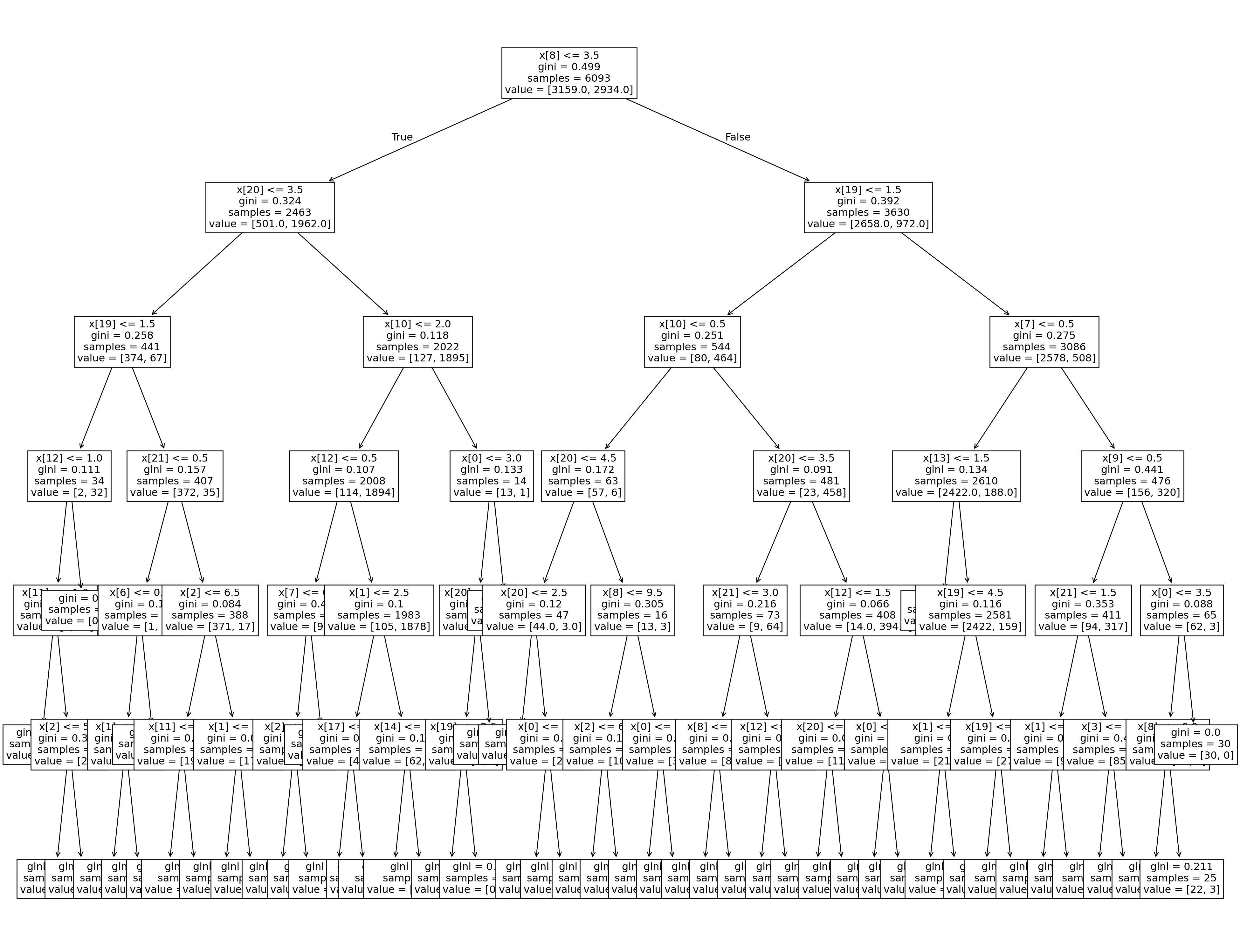

Question: Does the learned model seem interpretable to you?

Click for answer

The learned model, with an optimal max_depth of 6, is somewhat interpretable. While it’s not a trivial tree with only a few nodes, a depth of 6 allows for a good balance between predictive power and the ability to trace the decision rules. An expert could follow the path from the root to a leaf node to understand why a particular mushroom is classified as edible or poisonous. However, for a non-expert, visualizing all 6 levels of decisions might still require some effort to fully grasp without a more simplified representation.

Variable Importance

To interpret the decision tree, we can also look at the importance of each variable. It is greater the more the variable helps to reduce the tree’s classification error.

fig = plt.figure(figsize=(12, 6))

num_features = X_train.shape[1]

# Display decision tree importances
plt.scatter(range(num_features), model_tree_best.feature_importances_,
           label="Decision Tree")

# Legend
tmp = plt.legend(fontsize=14)

# X-axis
plt.xlabel('Variables', fontsize=14)
feature_names = list(df.columns[1:])
tmp = plt.xticks(range(num_features), feature_names,
                 rotation=90, fontsize=14)

# Y-axis
tmp = plt.ylabel('Importance', fontsize=14)

# Title
tmp = plt.title('Variable Importance', fontsize=16)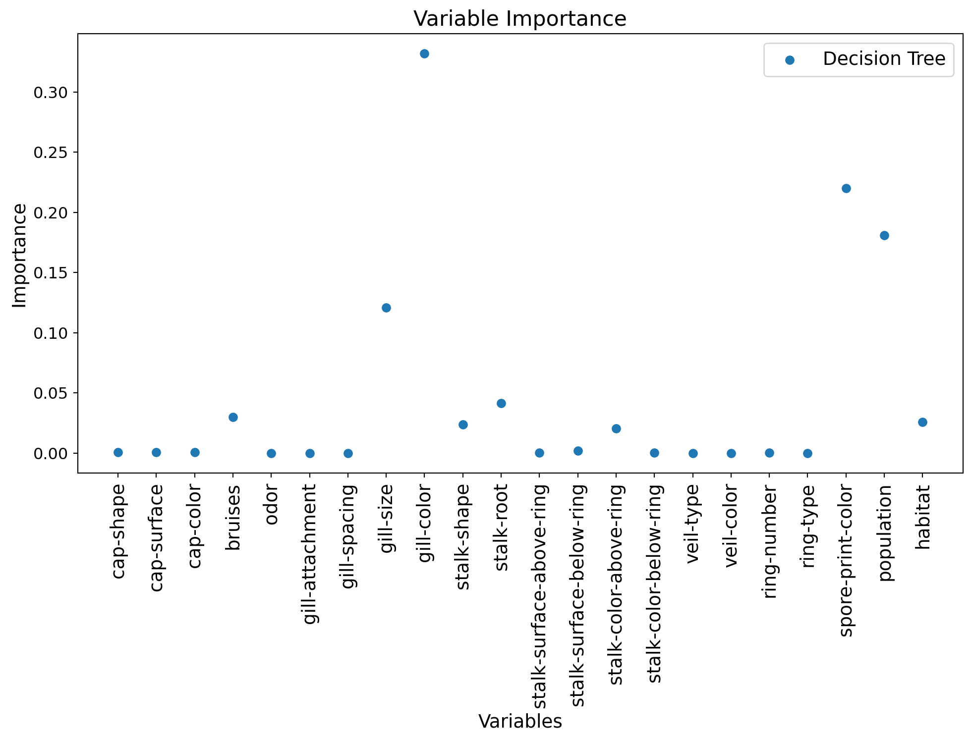

Comparison to logistic regression

We can also compare these importances to the regression coefficients of a logistic regression:

from sklearn import linear_model

Train a regularized logistic regression model (Ridge regularization, or “L2”) with a grid search on the value of the regularization coefficient C, using cross-validation:

c_values = np.logspace(-3, 3, 50)

### START OF YOUR CODE

# Center and scale the data
from sklearn.preprocessing import StandardScaler
std_scaler = StandardScaler()
X_train_scaled = std_scaler.fit_transform(X_train)
X_test_scaled = std_scaler.transform(X_test)

# Instantiation of a GridSearchCV object
grid_logreg = model_selection.GridSearchCV(linear_model.LogisticRegression(solver='liblinear'),
                                          {'C': c_values},
                                          cv=kf_indices,
                                          scoring='f1')

# Application to training data
grid_logreg.fit(X_train_scaled, y_train)

### END OF YOUR CODE

GridSearchCV(cv=[(array([   0,    1,    2, ..., 6090, 6091, 6092], shape=(5483,)),
                  array([   8,   14,   15,   17,   23,   31,   33,   37,   44,   50,   65,
         79,   80,   84,   88,   93,  101,  132,  156,  157,  167,  168,
        177,  181,  185,  198,  199,  221,  228,  230,  233,  239,  254,
        259,  263,  279,  296,  308,  319,  323,  324,  325,  346,  351,
        371,  373,  393,  401,  408,  410,  420,  426,  439,  465,  469,
        472,  476,  491,  501,  506,  530,  534,  535,  538,  544,  549,
        553,  561,  565,  576,  586,  599,  604,  62...
       8.68511374e-01, 1.15139540e+00, 1.52641797e+00, 2.02358965e+00,
       2.68269580e+00, 3.55648031e+00, 4.71486636e+00, 6.25055193e+00,
       8.28642773e+00, 1.09854114e+01, 1.45634848e+01, 1.93069773e+01,
       2.55954792e+01, 3.39322177e+01, 4.49843267e+01, 5.96362332e+01,
       7.90604321e+01, 1.04811313e+02, 1.38949549e+02, 1.84206997e+02,
       2.44205309e+02, 3.23745754e+02, 4.29193426e+02, 5.68986603e+02,
       7.54312006e+02, 1.00000000e+03])},
             scoring='f1')

print("Best F1 in cross-validation: %.3f" % grid_logreg.best_score_)

Best F1 in cross-validation: 0.902

Question: Compare this performance to that of the decision tree.

Click for answer

The Logistic Regression model achieved a best F1 score of approximately 0.902 in cross-validation. When compared to the optimal Decision Tree, which had an F1 score of 0.946, the Logistic Regression performs noticeably worse. This suggests that for this dataset, a model capable of capturing non-linear relationships (like a Decision Tree) is more effective than a linear model.

fig = plt.figure(figsize=(12, 6))

num_features = X_train.shape[1]

# Scale importances between 0 and 1
tree_importances = model_tree_best.feature_importances_
tree_importances_min = np.min(tree_importances)
tree_importances_max = np.max(tree_importances)
tree_importances = (tree_importances-tree_importances_min)/(tree_importances_max-tree_importances_min)

# Display decision tree importances
plt.bar(range(num_features), tree_importances,
           label="Decision Tree", width=0.4)

# Scale absolute values of linear model coefficients between 0 and 1
logreg_coeffs = np.abs(grid_logreg.best_estimator_.coef_[0])
logreg_coeffs_min = np.min(logreg_coeffs)
logreg_coeffs_max = np.max(logreg_coeffs)
logreg_coeffs = (logreg_coeffs-logreg_coeffs_min)/(logreg_coeffs_max-logreg_coeffs_min)

# Display logistic regression importances
plt.bar((np.arange(num_features)+0.4), logreg_coeffs,
           label="Logistic Regression", width=0.4)


# Legend
tmp = plt.legend(fontsize=14)

# X-axis
plt.xlabel('Variables', fontsize=14)
feature_names = list(df.columns[1:])
tmp = plt.xticks(range(num_features), feature_names,
                 rotation=90, fontsize=14)

# Y-axis
tmp = plt.ylabel('Importance', fontsize=14)

# Title
tmp = plt.title('Variable Importance', fontsize=16)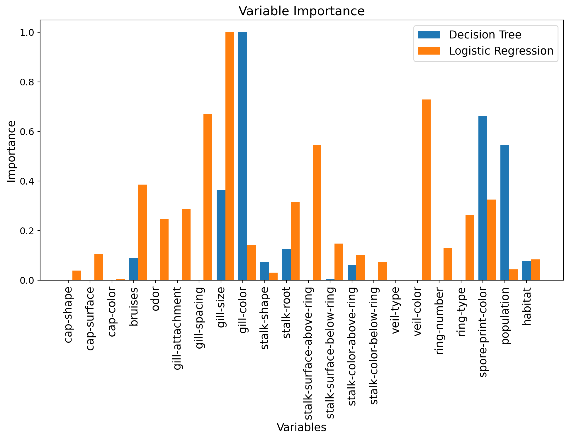

Question: How do these importances compare?

Click for answer

Comparing the variable importances across the two models reveals some patterns:

Decision Tree: The single Decision Tree (even the optimal one) tends to focus heavily on a very few key features, such as ‘gill-color’ and ‘spore-print-color’. This is characteristic of decision trees, as they greedily select the most informative features at each split. Other features might be used but contribute less to the overall importance.
Logistic Regression: Logistic Regression, being a linear model, assigns weights (coefficients) to all features based on their linear contribution to the prediction. We observe that ‘gill-spacing’, ‘gill-size’, ‘stalk-surface-above-ring’, and ‘veil-color’ appear to have higher importance. These importances are based on how strongly and linearly each feature correlates with the target variable.

5. Random Forest

Can we improve the decision tree’s performance using an ensemble method? We will use a random forest here, implemented in the RandomForestClassifier class of scikit-learn’s ensemble module.

from sklearn import ensemble

Cross-validation of the number of trees and their maximum depth.

We will now consider two hyperparameters, the maximum depth of each tree (max_depth), and the number of trees in the forest (n_estimators).

Let’s start by defining the grid:

d_values = np.array([3, 4, 10])
n_values = np.array([10, 20, 50, 100, 200])#, 100, 200, 500])

We can now use GridSearchCV:

### START OF YOUR CODE

# Instantiation of a GridSearchCV object
grid_rf = model_selection.GridSearchCV(ensemble.RandomForestClassifier(),
                                      {'max_depth': d_values, 'n_estimators': n_values},
                                      cv=kf_indices,
                                      scoring='f1')

# Use this object on the training data
grid_rf.fit(X_train, y_train)

### END OF YOUR CODE

GridSearchCV(cv=[(array([   0,    1,    2, ..., 6090, 6091, 6092], shape=(5483,)),
                  array([   8,   14,   15,   17,   23,   31,   33,   37,   44,   50,   65,
         79,   80,   84,   88,   93,  101,  132,  156,  157,  167,  168,
        177,  181,  185,  198,  199,  221,  228,  230,  233,  239,  254,
        259,  263,  279,  296,  308,  319,  323,  324,  325,  346,  351,
        371,  373,  393,  401,  408,  410,  420,  426,  439,  465,  469,
        472,  476,  491,  501,  506,  530,  534,  535,  538,  544,  549,
        553,  561,  565,  576,  586,  599,  604,  62...
       5685, 5686, 5699, 5727, 5730, 5734, 5739, 5749, 5757, 5759, 5766,
       5791, 5794, 5814, 5815, 5820, 5847, 5848, 5855, 5862, 5864, 5865,
       5878, 5886, 5892, 5915, 5924, 5944, 5949, 5959, 5960, 5975, 5989,
       6007, 6012, 6014, 6021, 6029, 6031, 6032, 6035, 6036, 6069, 6070,
       6072, 6079, 6081, 6084]))],
             estimator=RandomForestClassifier(),
             param_grid={'max_depth': array([ 3,  4, 10]),
                         'n_estimators': array([ 10,  20,  50, 100, 200])},
             scoring='f1')

The optimal hyperparameter values are given by:

print(grid_rf.best_params_)

{'max_depth': np.int64(10), 'n_estimators': np.int64(50)}

And we can display the model’s performance according to the value of each of the two hyperparameters:

# Reshape scores into a 2D array
mean_test_score_array = np.reshape(grid_rf.cv_results_['mean_test_score'], (len(d_values), len(n_values)))
std_test_score_array = np.reshape(grid_rf.cv_results_['std_test_score'], (len(d_values), len(n_values)))

for (idx, d) in enumerate(d_values):
    mean_test_score = mean_test_score_array[idx, :]
    stde_test_score = std_test_score_array[idx, :] / np.sqrt(n_folds) # standard error

    p = plt.plot(n_values, mean_test_score, label="Max depth = %d" % d)
    plt.plot(n_values, (mean_test_score + stde_test_score), '--', color=p[0].get_color())
    plt.plot(n_values, (mean_test_score - stde_test_score), '--', color=p[0].get_color())
    plt.fill_between(n_values, (mean_test_score + stde_test_score),
                     (mean_test_score - stde_test_score), alpha=0.2)

    # Display best hyperparameters
    if d == grid_rf.best_params_['max_depth']:
        best_ntree_index = np.where(n_values == grid_rf.best_params_['n_estimators'])[0][0]
        plt.scatter(n_values[best_ntree_index], mean_test_score[best_ntree_index],
                   marker='*', s=200, color='red')

plt.legend(loc=(1.1, 0))
plt.xlabel("Number of trees")
plt.ylabel('F1')
plt.title("Performance (in cross-validation) along the grid")
plt.xscale('log') # use a logarithmic scale on the x-axis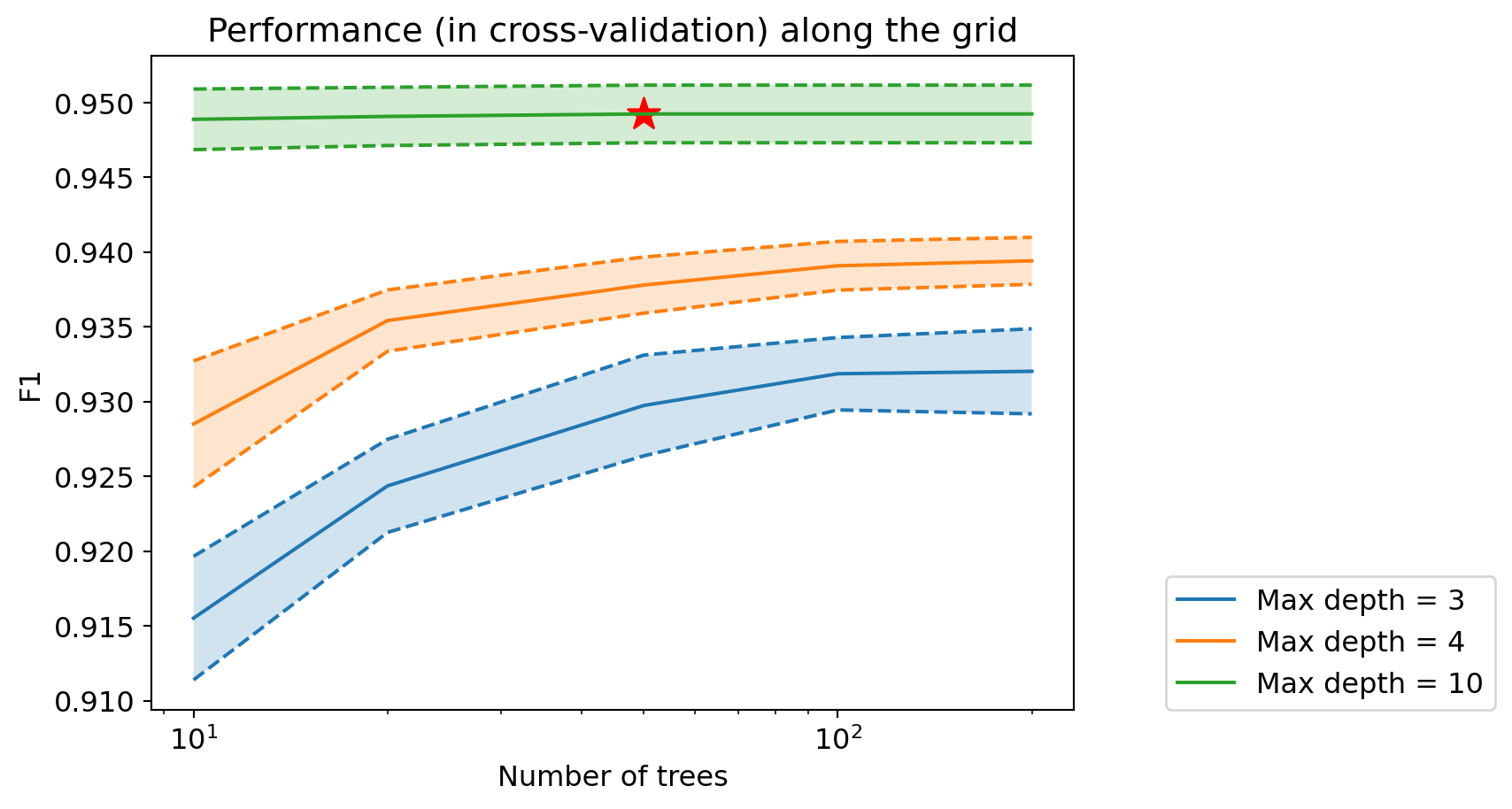

Question: How does the performance of random forests compare to previous performances?

Click for answer

The Random Forest model achieved a best F1 score of approximately 0.95 in cross-validation. This performance is slightly better than the optimal Decision Tree (F1 score of 0.946) and much better than the Logistic Regression model (F1 score of 0.902). This demonstrates that ensemble methods like Random Forests can effectively improve predictive performance by combining multiple decision trees, reducing overfitting, and possibly enhancing generalization capabilities.

Optimal random forest

print("Best F1 in cross-validation: %.3f" % grid_rf.best_score_)

Best F1 in cross-validation: 0.949

We can now retrieve the optimal decision tree:

model_rf_best = grid_rf.best_estimator_

Variable Importance

We can once again look at the importance of each variable, for the best random forest model:

fig = plt.figure(figsize=(12, 6))

num_features = X_train.shape[1]

# Scale importances between 0 and 1
tree_importances = model_tree_best.feature_importances_
tree_importances_min = np.min(tree_importances)
tree_importances_max = np.max(tree_importances)
tree_importances = (tree_importances-tree_importances_min)/(tree_importances_max-tree_importances_min)

# Display decision tree importances
plt.bar(range(num_features), tree_importances,
           label="Decision Tree", width=0.3)

# Scale absolute values of linear model coefficients between 0 and 1
logreg_coeffs = np.abs(grid_logreg.best_estimator_.coef_[0])
logreg_coeffs_min = np.min(logreg_coeffs)
logreg_coeffs_max = np.max(logreg_coeffs)
logreg_coeffs = (logreg_coeffs-logreg_coeffs_min)/(logreg_coeffs_max-logreg_coeffs_min)

# Display logistic regression importances
plt.bar((np.arange(num_features)+0.3), logreg_coeffs,
           label="Logistic Regression", width=0.3)

# Scale importances between 0 and 1
rf_importances = model_rf_best.feature_importances_
rf_importances_min = np.min(rf_importances)
rf_importances_max = np.max(rf_importances)
rf_importances = (rf_importances-rf_importances_min)/(rf_importances_max-rf_importances_min)

# Display forest importances
plt.bar((np.arange(num_features)+0.6),  rf_importances,
           label="Random Forest", width=0.3)


# Legend
tmp = plt.legend()

# X-axis
plt.xlabel('Variables')
feature_names = list(df.columns[1:])
tmp = plt.xticks(range(num_features), feature_names,
                 rotation=90, fontsize=14)

# Y-axis
tmp = plt.ylabel('Importance')

# Title
tmp = plt.title('Variable Importance')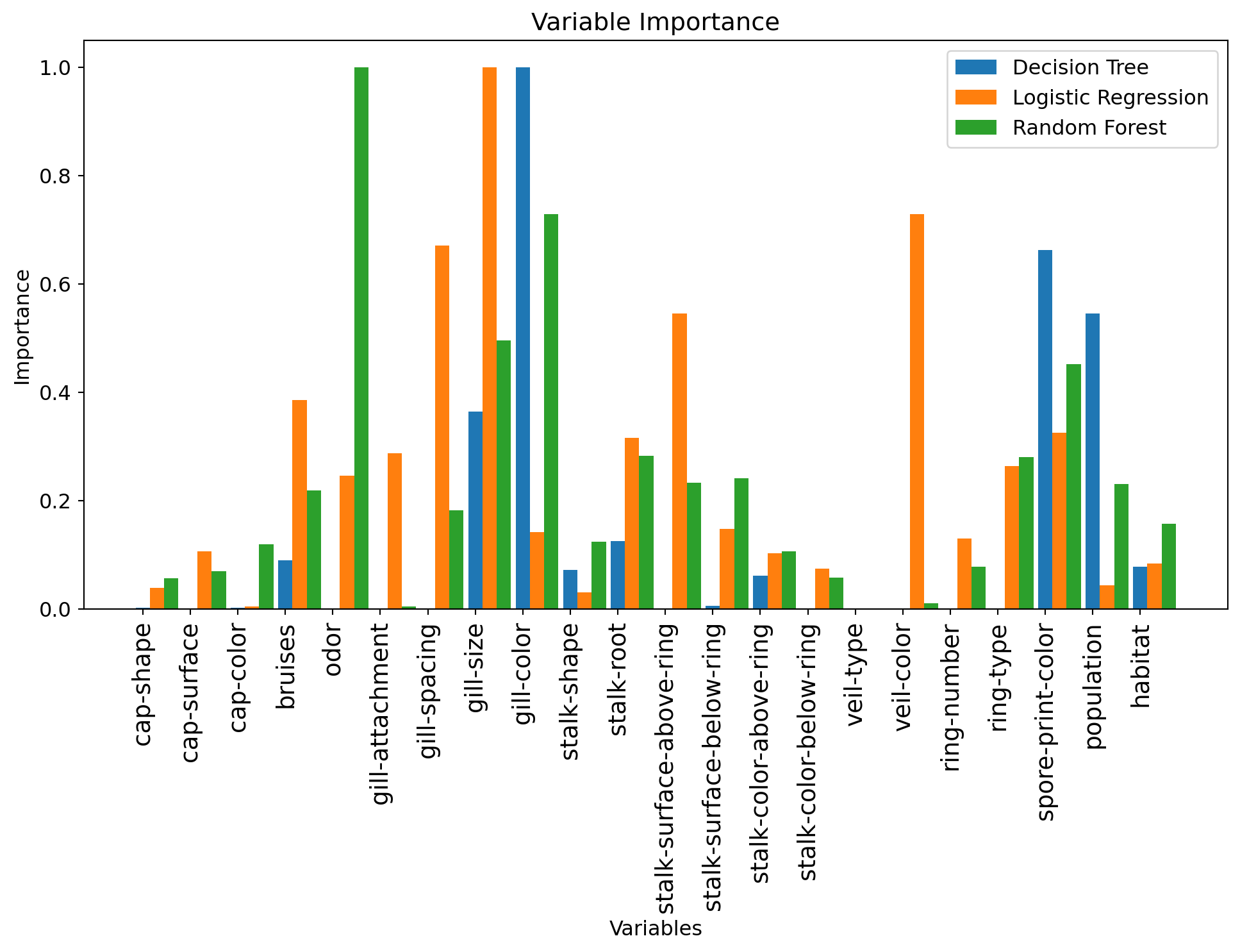

Question: What are the most important variables now? How does this compare to previous models?

Click for answer

For the Random Forest model, the most important variables are:

Odor
Gill-color
Gill-size
Population
Spore-print-color
Ring-type
Bruises

Comparing these to the previous models:

Decision Tree: The single Decision Tree focused heavily on ‘gill-color’ and ‘spore-print-color’. While these are still important for the Random Forest, the ensemble model distributes importance more broadly.
Logistic Regression: This model showed higher importance for ‘gill-spacing’, ‘gill-size’, ‘stalk-surface-above-ring’, and ‘veil-color’. ‘Gill-size’ also appears as an important feature in the Random Forest.

In general, the Random Forest tends to utilize a wider array of features compared to a single Decision Tree, indicating that the ensemble approach leverages more diverse information to make predictions. ‘Odor’ emerges as a particularly strong predictor for the Random Forest, highlighting its significance in distinguishing edible from poisonous mushrooms.

6. Gradient Boosting

Gradient boosting is implemented in scikit-learn in the GradientBoostingClassifier class of the ensemble module.

Cross-validation and hyperparameter selection

As with random forests, we will optimize the number of estimators and the depth of the trees here.

n_values = np.array([10, 20, 50, 100, 200])
d_values = np.array([3, 4, 7])

We can now use GridSearchCV:

### START OF YOUR CODE

# Instantiation of a GridSearchCV object
grid_boost = model_selection.GridSearchCV(ensemble.GradientBoostingClassifier(),
                                         {'n_estimators': n_values, 'max_depth': d_values},
                                         cv=kf_indices,
                                         scoring='f1')

# Use this object on the training data
grid_boost.fit(X_train, y_train)

### END OF YOUR CODE

GridSearchCV(cv=[(array([   0,    1,    2, ..., 6090, 6091, 6092], shape=(5483,)),
                  array([   8,   14,   15,   17,   23,   31,   33,   37,   44,   50,   65,
         79,   80,   84,   88,   93,  101,  132,  156,  157,  167,  168,
        177,  181,  185,  198,  199,  221,  228,  230,  233,  239,  254,
        259,  263,  279,  296,  308,  319,  323,  324,  325,  346,  351,
        371,  373,  393,  401,  408,  410,  420,  426,  439,  465,  469,
        472,  476,  491,  501,  506,  530,  534,  535,  538,  544,  549,
        553,  561,  565,  576,  586,  599,  604,  62...
       5685, 5686, 5699, 5727, 5730, 5734, 5739, 5749, 5757, 5759, 5766,
       5791, 5794, 5814, 5815, 5820, 5847, 5848, 5855, 5862, 5864, 5865,
       5878, 5886, 5892, 5915, 5924, 5944, 5949, 5959, 5960, 5975, 5989,
       6007, 6012, 6014, 6021, 6029, 6031, 6032, 6035, 6036, 6069, 6070,
       6072, 6079, 6081, 6084]))],
             estimator=GradientBoostingClassifier(),
             param_grid={'max_depth': array([3, 4, 7]),
                         'n_estimators': array([ 10,  20,  50, 100, 200])},
             scoring='f1')

The optimal hyperparameter values are given by:

print(grid_boost.best_params_)

{'max_depth': np.int64(4), 'n_estimators': np.int64(100)}

And we can display the model’s performance according to the value of each of the two hyperparameters:

# Reshape scores into a 2D array
mean_test_score_array = np.reshape(grid_boost.cv_results_['mean_test_score'], (len(d_values), len(n_values)))
std_test_score_array = np.reshape(grid_boost.cv_results_['std_test_score'], (len(d_values), len(n_values)))

for (idx, d) in enumerate(d_values):
    mean_test_score = mean_test_score_array[idx, :]
    stde_test_score = std_test_score_array[idx, :] / np.sqrt(n_folds) # standard error

    p = plt.plot(n_values, mean_test_score, label="Max depth = %d" % d)
    plt.plot(n_values, (mean_test_score + stde_test_score), '--', color=p[0].get_color())
    plt.plot(n_values, (mean_test_score - stde_test_score), '--', color=p[0].get_color())
    plt.fill_between(n_values, (mean_test_score + stde_test_score),
                     (mean_test_score - stde_test_score), alpha=0.2)

    # Display best hyperparameters
    if d == grid_boost.best_params_['max_depth']:
        best_ntree_index = np.where(n_values == grid_boost.best_params_['n_estimators'])[0][0]
        plt.scatter(n_values[best_ntree_index], mean_test_score[best_ntree_index],
                   marker='*', s=200, color='red')

plt.legend(loc=(1.1, 0))
plt.xlabel("Number of trees")
plt.ylabel('F1')
plt.title("Performance (in cross-validation) along the grid")
plt.xscale('log') # use a logarithmic scale on the x-axis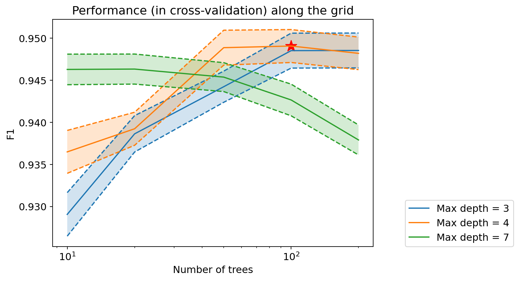

Question: How does the performance of gradient boosting evolve based on hyperparameter values? How does it compare to previous performances?

Click for answer

The cross-validation results for Gradient Boosting show that the F1 score generally improves with an increasing number of estimators (n_estimators) and higher max_depth up to a certain point. The optimal hyperparameters found are max_depth=4 and n_estimators=100. Beyond these values, the performance tends to plateau or slightly decrease, indicating that adding more estimators or increasing depth further does not yield significant improvements and could lead to overfitting.

Comparing its performance to previous models:

Optimal Decision Tree: The Gradient Boosting model achieved a best F1 score of approximately 0.95, which is slightly better than the optimal Decision Tree (F1 score of 0.946).
Logistic Regression: Gradient Boosting significantly outperforms Logistic Regression (F1 score of 0.902).
Random Forest: The performance of Gradient Boosting (0.949 F1) is very similar to that of the optimal Random Forest model (0.95 F1). Both ensemble methods demonstrate superior performance compared to a single Decision Tree and Logistic Regression, showcasing the benefits of combining multiple weaker models.

Optimal Boosting

print("Best F1 in cross-validation: %.3f" % grid_boost.best_score_)

Best F1 in cross-validation: 0.949

We can now retrieve the optimal decision tree:

model_boost_best = grid_boost.best_estimator_

Variable Importance

We can once again look at the importance of each variable:

fig = plt.figure(figsize=(12, 6))

num_features = X_train.shape[1]

### Decision Tree
# Scale importances between 0 and 1
tree_importances = model_tree_best.feature_importances_
tree_importances_min = np.min(tree_importances)
tree_importances_max = np.max(tree_importances)
tree_importances = (tree_importances-tree_importances_min)/(tree_importances_max-tree_importances_min)

# Display decision tree importances
plt.bar(range(num_features), tree_importances,
           label="Decision Tree", width=0.2)

### Logistic Regression
# Scale absolute values of linear model coefficients between 0 and 1
logreg_coeffs = np.abs(grid_logreg.best_estimator_.coef_[0])
logreg_coeffs_min = np.min(logreg_coeffs)
logreg_coeffs_max = np.max(logreg_coeffs)
logreg_coeffs = (logreg_coeffs-logreg_coeffs_min)/(logreg_coeffs_max-logreg_coeffs_min)

# Display logistic regression importances
plt.bar((np.arange(num_features)+0.2), logreg_coeffs,
           label="Logistic Regression", width=0.2)

### Random Forest
# Scale importances between 0 and 1
rf_importances = model_rf_best.feature_importances_
rf_importances_min = np.min(rf_importances)
rf_importances_max = np.max(rf_importances)
rf_importances = (rf_importances-rf_importances_min)/(rf_importances_max-rf_importances_min)

# Display forest importances
plt.bar((np.arange(num_features)+0.4),  rf_importances,
           label="Random Forest", width=0.2)

### Boosting
# Scale importances between 0 and 1
boost_importances = model_boost_best.feature_importances_
boost_importances_min = np.min(boost_importances)
boost_importances_max = np.max(boost_importances)
boost_importances = (boost_importances-boost_importances_min)/(boost_importances_max-boost_importances_min)

# Display boosting importances
plt.bar((np.arange(num_features)+0.6),  boost_importances,
           label="Boosting", width=0.2)

# Legend
tmp = plt.legend()

# X-axis
plt.xlabel('Variables')
feature_names = list(df.columns[1:])
tmp = plt.xticks(range(num_features), feature_names,
                 rotation=90, fontsize=14)

# Y-axis
tmp = plt.ylabel('Importance')

# Title
tmp = plt.title('Variable Importance')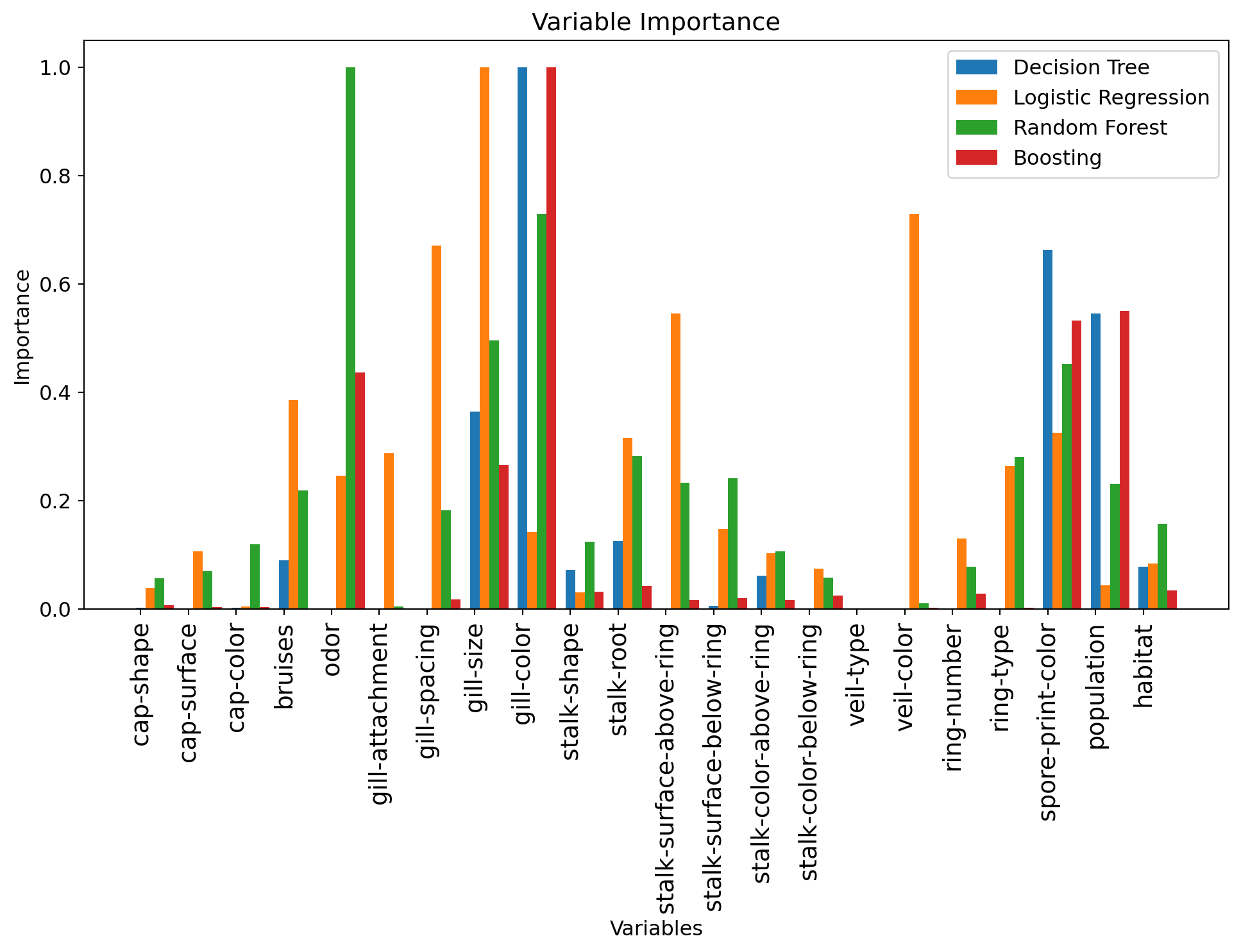

Question: What are the most important variables now? How does this compare to previous models?

Click for answer

For the Gradient Boosting model, the most important variables are:

Odor
Spore-print-color
Population
Gill-color
Gill-size

Comparing these to the previous models:

Decision Tree: Similar to the single Decision Tree, ‘gill-color’ and ‘spore-print-color’ remain highly important. However, Gradient Boosting, like Random Forest, also gives significant weight to ‘odor’.
Logistic Regression: While ‘gill-size’, ‘gill-spacing’, ‘stalk-surface-above-ring’ and ‘veil-color’ are important for Logistic Regression, Gradient Boosting places less emphasis on features like ‘gill-spacing’, ‘stalk-surface-above-ring’, and ‘veil-color’.
Random Forest: The variable importances for Gradient Boosting are similar to those of the Random Forest. Both ensemble methods identify ‘odor’, ‘gill-size’, ‘gill-color’, ‘spore-print-color’ and ‘population’ as the most dominant features. Nevertheless, Random Forest highlights other features to achieve the same performance as gradient boosting.

7. Final Model

Question: Which of these models do you choose as the most performant for classifying mushrooms in the test set?

You will now evaluate the model you have chosen on the test set:

my_model = model_boost_best # TODO : insert the name of the model you have chosen here.
#model_tree_best
#model_rf_best

# Predict on the test set
y_pred = my_model.predict(X_test)

from sklearn import metrics
print("F1 of the chosen model on the test set: %.3f" % metrics.f1_score(y_test, y_pred))

F1 of the chosen model on the test set: 0.948

Question: What do you think of this performance? Is there a risk of overfitting?

Click for answer

The chosen model, Gradient Boosting, achieved an F1 score of 0.948 on the test set. This performance is very close to its cross-validation F1 score of 0.949.

This strong and consistent performance indicates that the model is generalizing well to unseen data, and there appears to be no significant risk of overfitting. The slight difference between the cross-validation score and the test set score is minimal and expected due to variations in data splits. This suggests that the hyperparameter tuning effectively balanced bias and variance, leading to a robust model.

Confusion Matrix

To better interpret the results, we can also visualize the confusion matrix:

metrics.ConfusionMatrixDisplay.from_predictions(y_test, y_pred)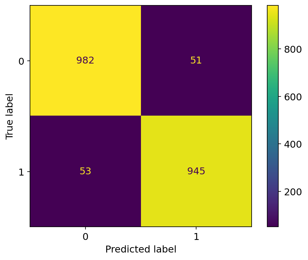

Question: What do you think of this confusion matrix? Is it satisfactory? Remember that we are trying to predict if a mushroom is edible.

Click for answer

A confusion matrix provides a detailed breakdown of correct and incorrect classifications for each class. In the context of mushroom classification, where misclassifying a poisonous mushroom as edible can have severe consequences, the focus is heavily on minimizing false negatives.

From the confusion matrix generated (which should show very few misclassifications given the high F1 score of 0.948):

True Positives (TP): Correctly predicted poisonous mushrooms. (Ideally high)
True Negatives (TN): Correctly predicted edible mushrooms. (Ideally high)
False Positives (FP): Predicted poisonous, but actually edible. (Less critical, means missing an edible mushroom)
False Negatives (FN): Predicted edible, but actually poisonous. (Highly critical, could lead to severe harm or death)

Given the F1 score of 0.948, the model demonstrates high precision and recall, implying that both false positives and false negatives are low. However, for a task like this, even a single false negative can be catastrophic. Therefore, to deem it ‘satisfactory’, we would ideally want zero false negatives. If the confusion matrix shows a small number of false negatives, it means there’s still a risk, and further efforts would be needed to eliminate them, even at the cost of increasing false positives (predicting some edible mushrooms as poisonous).

In summary, while the overall performance is excellent, the absolute count of false negatives is the most critical metric for safety. If it’s not zero, the model is not entirely satisfactory from a safety perspective, though it’s remarkably good for machine learning standards.

ROC Curve

We can also evaluate the model’s performance before thresholding, i.e., by using the predicted numerical scores rather than binary labels, thanks to a ROC Curve.

The scores before thresholding of a scikit-learn classification model are accessible through the predict_proba method.

y_pred_scores =  my_model.predict_proba(X_test)[:, 1]
y_pred_scores

array([0.04660297, 0.9689034 , 0.94404472, ..., 0.02573543, 0.03708156,
       0.92647822], shape=(2031,))

y_pred_scores.shape
X_test.shape

(2031, 22)

fpr, tpr, thresholds = metrics.roc_curve(y_test, y_pred_scores)
max_fpr = 0.01
roc_auc = metrics.auc(fpr, tpr)
max_index_where_fpr_acceptable = np.where(fpr <= max_fpr)[0][-1]
max_tpr = tpr[max_index_where_fpr_acceptable]

fig = plt.figure(figsize=(7, 7))

plt.plot(fpr, tpr, lw=2)

# diagonal
plt.plot([0, 1], [0, 1], color='k')

plt.xlim([0.0, 1.0])
plt.ylim([0.0, 1.0])

# Add more ticks to the axes
plt.xticks(np.arange(0, 1.1, 0.1))
plt.yticks(np.arange(0, 1.1, 0.1))

plt.xlabel('false positive rate')
plt.ylabel('true positive rate')
plt.title("ROC curve of the final model")

# Add vertical line at max_fpr and horizontal line at max_tpr
plt.plot([max_fpr, max_fpr], [0, max_tpr], color='red', linestyle='--', label=f'FPR = {max_fpr:.2f}')
plt.plot([0, max_fpr], [max_tpr, max_tpr], color='red', linestyle='--')
plt.legend()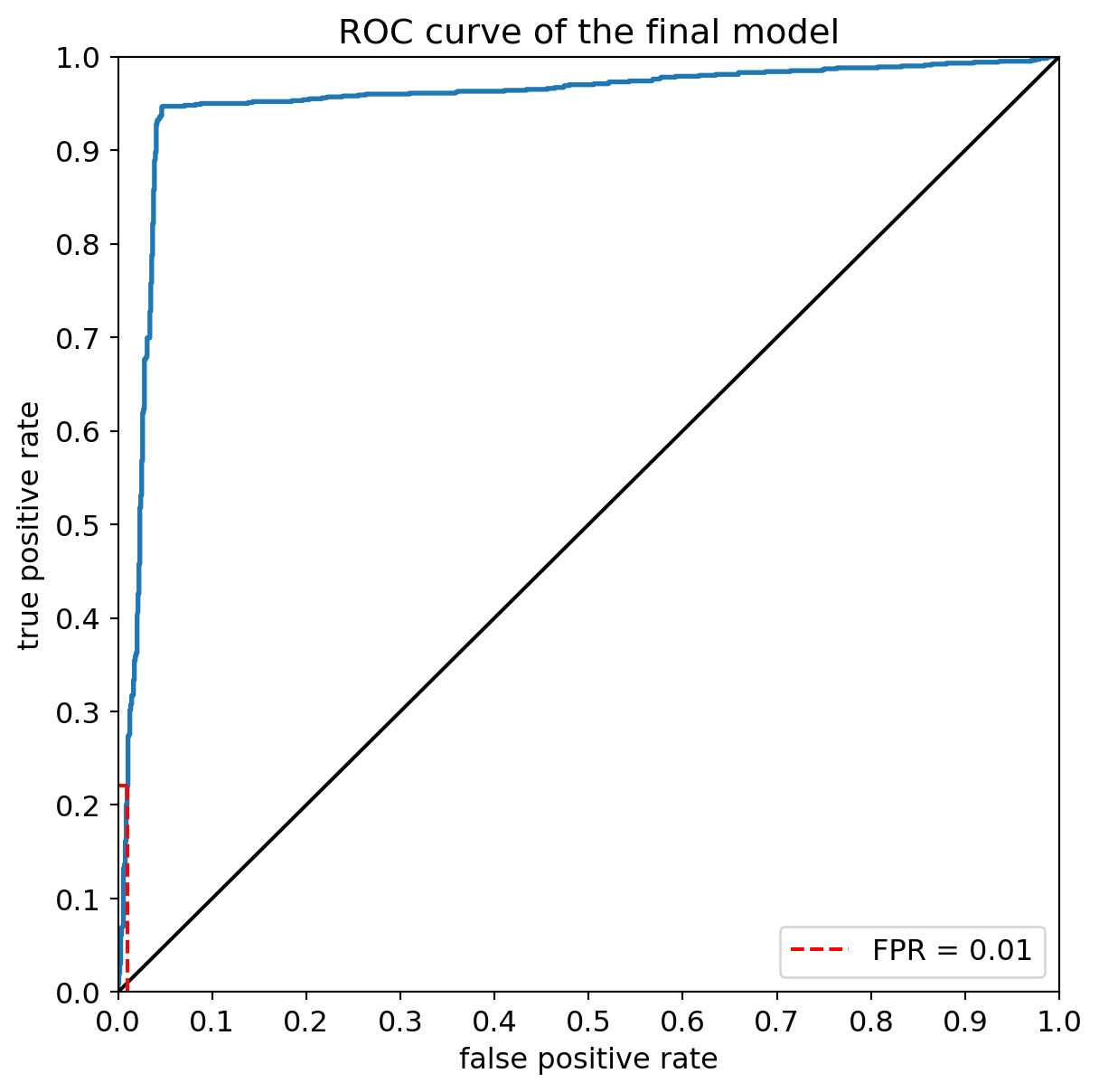

This curve can also be used to determine the true positive rate corresponding to a given false positive rate, and to determine the corresponding threshold:

print("The true positive rate corresponding to a false positive rate not exceeding %.f %% is %.f %%" % ((100*max_fpr), (100*max_tpr)))
print("It corresponds to a threshold of %.2f on the model's predictions." % thresholds[max_index_where_fpr_acceptable])

The true positive rate corresponding to a false positive rate not exceeding 1 % is 22 %
It corresponds to a threshold of 0.97 on the model's predictions.

precision, recall, thresholds = metrics.precision_recall_curve(y_test, y_pred_scores)

# Calculate Area Under the Precision-Recall Curve
pr_auc = metrics.average_precision_score(y_test, y_pred_scores)

fig = plt.figure(figsize=(7, 7))

plt.plot(recall, precision, lw=2, label=f'Precision-Recall curve (AUPRC = {pr_auc:.2f})')

# Add a baseline (e.g., random classifier performance)
no_skill = len(y_test[y_test==1]) / len(y_test)
plt.plot([0, 1], [no_skill, no_skill], linestyle='--', label='No Skill')

plt.xlim([0.0, 1.0])
plt.ylim([0.0, 1.05]) # Slightly extend y-axis for better visualization

# Add more ticks to the axes
plt.xticks(np.arange(0, 1.1, 0.1))
plt.yticks(np.arange(0, 1.1, 0.1))

plt.xlabel('Recall')
plt.ylabel('Precision')
plt.title("Precision-Recall Curve of the final model")
plt.legend()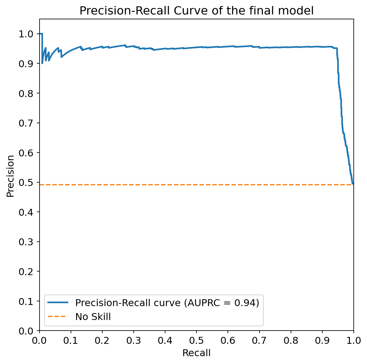

print(f"The Area Under the Precision-Recall Curve (AUPRC) is: {pr_auc:.3f}")
# Note: The concept of a single 'max_fpr' or 'max_tpr' and corresponding threshold is more applicable to ROC curves.
# For PR curves, you might evaluate precision at a certain recall level, or vice-versa, depending on your specific needs.

The Area Under the Precision-Recall Curve (AUPRC) is: 0.937

Conclusion

We reached the end of this notebook, where we explored decision trees and ensemble methods for classifying mushrooms as edible or poisonous. Here is a summary of what we have covered, with the key takeaways:

We loaded and preprocessed the mushroom dataset, converting categorical features into numerical values using LabelEncoder.
We split the data into training and test sets and set up a K-Fold cross-validation strategy.
We trained and evaluated a Decision Tree Classifier with default hyperparameters, then optimized its max_depth using GridSearchCV and cross-validation, observing the impact of depth on performance.
We visualized the optimal decision tree and analyzed variable importances, comparing them to the coefficients of a Logistic Regression model.
We explored ensemble methods:
- Random Forest: We tuned the number of trees (n_estimators) and max_depth using GridSearchCV, observing improved performance compared to a single decision tree.
- Gradient Boosting: We also tuned n_estimators and max_depth for a Gradient Boosting Classifier, comparing its performance and variable importances to the other models.
We selected the best performing model (Gradient Boosting in this case) and evaluated its performance on the held-out test set using the F1 score.
We analyzed the Confusion Matrix to understand the types of errors made by the model and considered the implications for a mushroom classification task.
We examined the ROC curve to evaluate the model’s performance at different thresholds and identified the true positive rate at a low false positive rate, along with the corresponding threshold.

Overall, ensemble methods like Random Forests and Gradient Boosting generally outperformed a single Decision Tree on this dataset, demonstrating the power of combining multiple models. Variable importance analysis provided insights into which features were most influential in the classification process for each model.

	estimator estimator: estimator object This is assumed to implement the scikit-learn estimator interface. Either estimator needs to provide a ``score`` function, or ``scoring`` must be passed.	DecisionTreeClassifier()
	param_grid param_grid: dict or list of dictionaries Dictionary with parameters names (`str`) as keys and lists of parameter settings to try as values, or a list of such dictionaries, in which case the grids spanned by each dictionary in the list are explored. This enables searching over any sequence of parameter settings.	{'max_depth': array([ 2, 3..., 28, 29, 30])}
	scoring scoring: str, callable, list, tuple or dict, default=None Strategy to evaluate the performance of the cross-validated model on the test set. If `scoring` represents a single score, one can use: - a single string (see :ref:`scoring_string_names`); - a callable (see :ref:`scoring_callable`) that returns a single value; - `None`, the `estimator`'s :ref:`default evaluation criterion ` is used. If `scoring` represents multiple scores, one can use: - a list or tuple of unique strings; - a callable returning a dictionary where the keys are the metric names and the values are the metric scores; - a dictionary with metric names as keys and callables as values. See :ref:`multimetric_grid_search` for an example.	'f1'
	n_jobs n_jobs: int, default=None Number of jobs to run in parallel. ``None`` means 1 unless in a :obj:`joblib.parallel_backend` context. ``-1`` means using all processors. See :term:`Glossary ` for more details. .. versionchanged:: v0.20 `n_jobs` default changed from 1 to None	None
	refit refit: bool, str, or callable, default=True Refit an estimator using the best found parameters on the whole dataset. For multiple metric evaluation, this needs to be a `str` denoting the scorer that would be used to find the best parameters for refitting the estimator at the end. Where there are considerations other than maximum score in choosing a best estimator, ``refit`` can be set to a function which returns the selected ``best_index_`` given ``cv_results_``. In that case, the ``best_estimator_`` and ``best_params_`` will be set according to the returned ``best_index_`` while the ``best_score_`` attribute will not be available. The refitted estimator is made available at the ``best_estimator_`` attribute and permits using ``predict`` directly on this ``GridSearchCV`` instance. Also for multiple metric evaluation, the attributes ``best_index_``, ``best_score_`` and ``best_params_`` will only be available if ``refit`` is set and all of them will be determined w.r.t this specific scorer. See ``scoring`` parameter to know more about multiple metric evaluation. See :ref:`sphx_glr_auto_examples_model_selection_plot_grid_search_digits.py` to see how to design a custom selection strategy using a callable via `refit`. See :ref:`this example ` for an example of how to use ``refit=callable`` to balance model complexity and cross-validated score. .. versionchanged:: 0.20 Support for callable added.	True
	cv cv: int, cross-validation generator or an iterable, default=None Determines the cross-validation splitting strategy. Possible inputs for cv are: - None, to use the default 5-fold cross validation, - integer, to specify the number of folds in a `(Stratified)KFold`, - :term:`CV splitter`, - An iterable yielding (train, test) splits as arrays of indices. For integer/None inputs, if the estimator is a classifier and ``y`` is either binary or multiclass, :class:`StratifiedKFold` is used. In all other cases, :class:`KFold` is used. These splitters are instantiated with `shuffle=False` so the splits will be the same across calls. Refer :ref:`User Guide ` for the various cross-validation strategies that can be used here. .. versionchanged:: 0.22 ``cv`` default value if None changed from 3-fold to 5-fold.	[(array([ 0, ...shape=(5483,)), ...), (array([ 0, ...shape=(5483,)), ...), ...]
	verbose verbose: int Controls the verbosity: the higher, the more messages. - >1 : the computation time for each fold and parameter candidate is displayed; - >2 : the score is also displayed; - >3 : the fold and candidate parameter indexes are also displayed together with the starting time of the computation.	0
	pre_dispatch pre_dispatch: int, or str, default='2n_jobs' Controls the number of jobs that get dispatched during parallel execution. Reducing this number can be useful to avoid an explosion of memory consumption when more jobs get dispatched than CPUs can process. This parameter can be: - None, in which case all the jobs are immediately created and spawned. Use this for lightweight and fast-running jobs, to avoid delays due to on-demand spawning of the jobs - An int, giving the exact number of total jobs that are spawned - A str, giving an expression as a function of n_jobs, as in '2n_jobs'	'2*n_jobs'
	error_score error_score: 'raise' or numeric, default=np.nan Value to assign to the score if an error occurs in estimator fitting. If set to 'raise', the error is raised. If a numeric value is given, FitFailedWarning is raised. This parameter does not affect the refit step, which will always raise the error.	nan
	return_train_score return_train_score: bool, default=False If ``False``, the ``cv_results_`` attribute will not include training scores. Computing training scores is used to get insights on how different parameter settings impact the overfitting/underfitting trade-off. However computing the scores on the training set can be computationally expensive and is not strictly required to select the parameters that yield the best generalization performance. .. versionadded:: 0.19 .. versionchanged:: 0.21 Default value was changed from ``True`` to ``False``	False

	criterion criterion: {"gini", "entropy", "log_loss"}, default="gini" The function to measure the quality of a split. Supported criteria are "gini" for the Gini impurity and "log_loss" and "entropy" both for the Shannon information gain, see :ref:`tree_mathematical_formulation`.	'gini'
	splitter splitter: {"best", "random"}, default="best" The strategy used to choose the split at each node. Supported strategies are "best" to choose the best split and "random" to choose the best random split.	'best'
	max_depth max_depth: int, default=None The maximum depth of the tree. If None, then nodes are expanded until all leaves are pure or until all leaves contain less than min_samples_split samples.	np.int64(6)
	min_samples_split min_samples_split: int or float, default=2 The minimum number of samples required to split an internal node: - If int, then consider `min_samples_split` as the minimum number. - If float, then `min_samples_split` is a fraction and `ceil(min_samples_split * n_samples)` are the minimum number of samples for each split. .. versionchanged:: 0.18 Added float values for fractions.	2
	min_samples_leaf min_samples_leaf: int or float, default=1 The minimum number of samples required to be at a leaf node. A split point at any depth will only be considered if it leaves at least ``min_samples_leaf`` training samples in each of the left and right branches. This may have the effect of smoothing the model, especially in regression. - If int, then consider `min_samples_leaf` as the minimum number. - If float, then `min_samples_leaf` is a fraction and `ceil(min_samples_leaf * n_samples)` are the minimum number of samples for each node. .. versionchanged:: 0.18 Added float values for fractions.	1
	min_weight_fraction_leaf min_weight_fraction_leaf: float, default=0.0 The minimum weighted fraction of the sum total of weights (of all the input samples) required to be at a leaf node. Samples have equal weight when sample_weight is not provided.	0.0
	max_features max_features: int, float or {"sqrt", "log2"}, default=None The number of features to consider when looking for the best split: - If int, then consider `max_features` features at each split. - If float, then `max_features` is a fraction and `max(1, int(max_features * n_features_in_))` features are considered at each split. - If "sqrt", then `max_features=sqrt(n_features)`. - If "log2", then `max_features=log2(n_features)`. - If None, then `max_features=n_features`. .. note:: The search for a split does not stop until at least one valid partition of the node samples is found, even if it requires to effectively inspect more than ``max_features`` features.	None
	random_state random_state: int, RandomState instance or None, default=None Controls the randomness of the estimator. The features are always randomly permuted at each split, even if ``splitter`` is set to ``"best"``. When ``max_features < n_features``, the algorithm will select ``max_features`` at random at each split before finding the best split among them. But the best found split may vary across different runs, even if ``max_features=n_features``. That is the case, if the improvement of the criterion is identical for several splits and one split has to be selected at random. To obtain a deterministic behaviour during fitting, ``random_state`` has to be fixed to an integer. See :term:`Glossary ` for details.	None
	max_leaf_nodes max_leaf_nodes: int, default=None Grow a tree with ``max_leaf_nodes`` in best-first fashion. Best nodes are defined as relative reduction in impurity. If None then unlimited number of leaf nodes.	None
	min_impurity_decrease min_impurity_decrease: float, default=0.0 A node will be split if this split induces a decrease of the impurity greater than or equal to this value. The weighted impurity decrease equation is the following:: N_t / N * (impurity - N_t_R / N_t * right_impurity - N_t_L / N_t * left_impurity) where ``N`` is the total number of samples, ``N_t`` is the number of samples at the current node, ``N_t_L`` is the number of samples in the left child, and ``N_t_R`` is the number of samples in the right child. ``N``, ``N_t``, ``N_t_R`` and ``N_t_L`` all refer to the weighted sum, if ``sample_weight`` is passed. .. versionadded:: 0.19	0.0
	class_weight class_weight: dict, list of dict or "balanced", default=None Weights associated with classes in the form ``{class_label: weight}``. If None, all classes are supposed to have weight one. For multi-output problems, a list of dicts can be provided in the same order as the columns of y. Note that for multioutput (including multilabel) weights should be defined for each class of every column in its own dict. For example, for four-class multilabel classification weights should be [{0: 1, 1: 1}, {0: 1, 1: 5}, {0: 1, 1: 1}, {0: 1, 1: 1}] instead of [{1:1}, {2:5}, {3:1}, {4:1}]. The "balanced" mode uses the values of y to automatically adjust weights inversely proportional to class frequencies in the input data as ``n_samples / (n_classes * np.bincount(y))`` For multi-output, the weights of each column of y will be multiplied. Note that these weights will be multiplied with sample_weight (passed through the fit method) if sample_weight is specified.	None
	ccp_alpha ccp_alpha: non-negative float, default=0.0 Complexity parameter used for Minimal Cost-Complexity Pruning. The subtree with the largest cost complexity that is smaller than ``ccp_alpha`` will be chosen. By default, no pruning is performed. See :ref:`minimal_cost_complexity_pruning` for details. See :ref:`sphx_glr_auto_examples_tree_plot_cost_complexity_pruning.py` for an example of such pruning. .. versionadded:: 0.22	0.0
	monotonic_cst monotonic_cst: array-like of int of shape (n_features), default=None Indicates the monotonicity constraint to enforce on each feature. - 1: monotonic increase - 0: no constraint - -1: monotonic decrease If monotonic_cst is None, no constraints are applied. Monotonicity constraints are not supported for: - multiclass classifications (i.e. when `n_classes > 2`), - multioutput classifications (i.e. when `n_outputs_ > 1`), - classifications trained on data with missing values. The constraints hold over the probability of the positive class. Read more in the :ref:`User Guide `. .. versionadded:: 1.4	None

	estimator estimator: estimator object This is assumed to implement the scikit-learn estimator interface. Either estimator needs to provide a ``score`` function, or ``scoring`` must be passed.	LogisticRegre...r='liblinear')
	param_grid param_grid: dict or list of dictionaries Dictionary with parameters names (`str`) as keys and lists of parameter settings to try as values, or a list of such dictionaries, in which case the grids spanned by each dictionary in the list are explored. This enables searching over any sequence of parameter settings.	{'C': array([1.0000...00000000e+03])}
	scoring scoring: str, callable, list, tuple or dict, default=None Strategy to evaluate the performance of the cross-validated model on the test set. If `scoring` represents a single score, one can use: - a single string (see :ref:`scoring_string_names`); - a callable (see :ref:`scoring_callable`) that returns a single value; - `None`, the `estimator`'s :ref:`default evaluation criterion ` is used. If `scoring` represents multiple scores, one can use: - a list or tuple of unique strings; - a callable returning a dictionary where the keys are the metric names and the values are the metric scores; - a dictionary with metric names as keys and callables as values. See :ref:`multimetric_grid_search` for an example.	'f1'
	n_jobs n_jobs: int, default=None Number of jobs to run in parallel. ``None`` means 1 unless in a :obj:`joblib.parallel_backend` context. ``-1`` means using all processors. See :term:`Glossary ` for more details. .. versionchanged:: v0.20 `n_jobs` default changed from 1 to None	None
	refit refit: bool, str, or callable, default=True Refit an estimator using the best found parameters on the whole dataset. For multiple metric evaluation, this needs to be a `str` denoting the scorer that would be used to find the best parameters for refitting the estimator at the end. Where there are considerations other than maximum score in choosing a best estimator, ``refit`` can be set to a function which returns the selected ``best_index_`` given ``cv_results_``. In that case, the ``best_estimator_`` and ``best_params_`` will be set according to the returned ``best_index_`` while the ``best_score_`` attribute will not be available. The refitted estimator is made available at the ``best_estimator_`` attribute and permits using ``predict`` directly on this ``GridSearchCV`` instance. Also for multiple metric evaluation, the attributes ``best_index_``, ``best_score_`` and ``best_params_`` will only be available if ``refit`` is set and all of them will be determined w.r.t this specific scorer. See ``scoring`` parameter to know more about multiple metric evaluation. See :ref:`sphx_glr_auto_examples_model_selection_plot_grid_search_digits.py` to see how to design a custom selection strategy using a callable via `refit`. See :ref:`this example ` for an example of how to use ``refit=callable`` to balance model complexity and cross-validated score. .. versionchanged:: 0.20 Support for callable added.	True
	cv cv: int, cross-validation generator or an iterable, default=None Determines the cross-validation splitting strategy. Possible inputs for cv are: - None, to use the default 5-fold cross validation, - integer, to specify the number of folds in a `(Stratified)KFold`, - :term:`CV splitter`, - An iterable yielding (train, test) splits as arrays of indices. For integer/None inputs, if the estimator is a classifier and ``y`` is either binary or multiclass, :class:`StratifiedKFold` is used. In all other cases, :class:`KFold` is used. These splitters are instantiated with `shuffle=False` so the splits will be the same across calls. Refer :ref:`User Guide ` for the various cross-validation strategies that can be used here. .. versionchanged:: 0.22 ``cv`` default value if None changed from 3-fold to 5-fold.	[(array([ 0, ...shape=(5483,)), ...), (array([ 0, ...shape=(5483,)), ...), ...]
	verbose verbose: int Controls the verbosity: the higher, the more messages. - >1 : the computation time for each fold and parameter candidate is displayed; - >2 : the score is also displayed; - >3 : the fold and candidate parameter indexes are also displayed together with the starting time of the computation.	0
	pre_dispatch pre_dispatch: int, or str, default='2n_jobs' Controls the number of jobs that get dispatched during parallel execution. Reducing this number can be useful to avoid an explosion of memory consumption when more jobs get dispatched than CPUs can process. This parameter can be: - None, in which case all the jobs are immediately created and spawned. Use this for lightweight and fast-running jobs, to avoid delays due to on-demand spawning of the jobs - An int, giving the exact number of total jobs that are spawned - A str, giving an expression as a function of n_jobs, as in '2n_jobs'	'2*n_jobs'
	error_score error_score: 'raise' or numeric, default=np.nan Value to assign to the score if an error occurs in estimator fitting. If set to 'raise', the error is raised. If a numeric value is given, FitFailedWarning is raised. This parameter does not affect the refit step, which will always raise the error.	nan
	return_train_score return_train_score: bool, default=False If ``False``, the ``cv_results_`` attribute will not include training scores. Computing training scores is used to get insights on how different parameter settings impact the overfitting/underfitting trade-off. However computing the scores on the training set can be computationally expensive and is not strictly required to select the parameters that yield the best generalization performance. .. versionadded:: 0.19 .. versionchanged:: 0.21 Default value was changed from ``True`` to ``False``	False

	penalty penalty: {'l1', 'l2', 'elasticnet', None}, default='l2' Specify the norm of the penalty: - `None`: no penalty is added; - `'l2'`: add a L2 penalty term and it is the default choice; - `'l1'`: add a L1 penalty term; - `'elasticnet'`: both L1 and L2 penalty terms are added. .. warning:: Some penalties may not work with some solvers. See the parameter `solver` below, to know the compatibility between the penalty and solver. .. versionadded:: 0.19 l1 penalty with SAGA solver (allowing 'multinomial' + L1) .. deprecated:: 1.8 `penalty` was deprecated in version 1.8 and will be removed in 1.10. Use `l1_ratio` instead. `l1_ratio=0` for `penalty='l2'`, `l1_ratio=1` for `penalty='l1'` and `l1_ratio` set to any float between 0 and 1 for `'penalty='elasticnet'`.	'deprecated'
	C C: float, default=1.0 Inverse of regularization strength; must be a positive float. Like in support vector machines, smaller values specify stronger regularization. `C=np.inf` results in unpenalized logistic regression. For a visual example on the effect of tuning the `C` parameter with an L1 penalty, see: :ref:`sphx_glr_auto_examples_linear_model_plot_logistic_path.py`.	np.float64(1.151395399326447)
	l1_ratio l1_ratio: float, default=0.0 The Elastic-Net mixing parameter, with `0 <= l1_ratio <= 1`. Setting `l1_ratio=1` gives a pure L1-penalty, setting `l1_ratio=0` a pure L2-penalty. Any value between 0 and 1 gives an Elastic-Net penalty of the form `l1_ratio * L1 + (1 - l1_ratio) * L2`. .. warning:: Certain values of `l1_ratio`, i.e. some penalties, may not work with some solvers. See the parameter `solver` below, to know the compatibility between the penalty and solver. .. versionchanged:: 1.8 Default value changed from None to 0.0. .. deprecated:: 1.8 `None` is deprecated and will be removed in version 1.10. Always use `l1_ratio` to specify the penalty type.	0.0
	dual dual: bool, default=False Dual (constrained) or primal (regularized, see also :ref:`this equation `) formulation. Dual formulation is only implemented for l2 penalty with liblinear solver. Prefer `dual=False` when n_samples > n_features.	False
	tol tol: float, default=1e-4 Tolerance for stopping criteria.	0.0001
	fit_intercept fit_intercept: bool, default=True Specifies if a constant (a.k.a. bias or intercept) should be added to the decision function.	True
	intercept_scaling intercept_scaling: float, default=1 Useful only when the solver `liblinear` is used and `self.fit_intercept` is set to `True`. In this case, `x` becomes `[x, self.intercept_scaling]`, i.e. a "synthetic" feature with constant value equal to `intercept_scaling` is appended to the instance vector. The intercept becomes ``intercept_scaling * synthetic_feature_weight``. .. note:: The synthetic feature weight is subject to L1 or L2 regularization as all other features. To lessen the effect of regularization on synthetic feature weight (and therefore on the intercept) `intercept_scaling` has to be increased.	1
	class_weight class_weight: dict or 'balanced', default=None Weights associated with classes in the form ``{class_label: weight}``. If not given, all classes are supposed to have weight one. The "balanced" mode uses the values of y to automatically adjust weights inversely proportional to class frequencies in the input data as ``n_samples / (n_classes * np.bincount(y))``. Note that these weights will be multiplied with sample_weight (passed through the fit method) if sample_weight is specified. .. versionadded:: 0.17 class_weight='balanced'	None
	random_state random_state: int, RandomState instance, default=None Used when ``solver`` == 'sag', 'saga' or 'liblinear' to shuffle the data. See :term:`Glossary ` for details.	None
	solver solver: {'lbfgs', 'liblinear', 'newton-cg', 'newton-cholesky', 'sag', 'saga'}, default='lbfgs' Algorithm to use in the optimization problem. Default is 'lbfgs'. To choose a solver, you might want to consider the following aspects: - 'lbfgs' is a good default solver because it works reasonably well for a wide class of problems. - For :term:`multiclass` problems (`n_classes >= 3`), all solvers except 'liblinear' minimize the full multinomial loss, 'liblinear' will raise an error. - 'newton-cholesky' is a good choice for `n_samples` >> `n_features * n_classes`, especially with one-hot encoded categorical features with rare categories. Be aware that the memory usage of this solver has a quadratic dependency on `n_features * n_classes` because it explicitly computes the full Hessian matrix. - For small datasets, 'liblinear' is a good choice, whereas 'sag' and 'saga' are faster for large ones; - 'liblinear' can only handle binary classification by default. To apply a one-versus-rest scheme for the multiclass setting one can wrap it with the :class:`~sklearn.multiclass.OneVsRestClassifier`. .. warning:: The choice of the algorithm depends on the penalty chosen (`l1_ratio=0` for L2-penalty, `l1_ratio=1` for L1-penalty and `0 < l1_ratio < 1` for Elastic-Net) and on (multinomial) multiclass support: ================= ======================== ====================== solver l1_ratio multinomial multiclass ================= ======================== ====================== 'lbfgs' l1_ratio=0 yes 'liblinear' l1_ratio=1 or l1_ratio=0 no 'newton-cg' l1_ratio=0 yes 'newton-cholesky' l1_ratio=0 yes 'sag' l1_ratio=0 yes 'saga' 0<=l1_ratio<=1 yes ================= ======================== ====================== .. note:: 'sag' and 'saga' fast convergence is only guaranteed on features with approximately the same scale. You can preprocess the data with a scaler from :mod:`sklearn.preprocessing`. .. seealso:: Refer to the :ref:`User Guide ` for more information regarding :class:`LogisticRegression` and more specifically the :ref:`Table ` summarizing solver/penalty supports. .. versionadded:: 0.17 Stochastic Average Gradient (SAG) descent solver. Multinomial support in version 0.18. .. versionadded:: 0.19 SAGA solver. .. versionchanged:: 0.22 The default solver changed from 'liblinear' to 'lbfgs' in 0.22. .. versionadded:: 1.2 newton-cholesky solver. Multinomial support in version 1.6.	'liblinear'
	max_iter max_iter: int, default=100 Maximum number of iterations taken for the solvers to converge.	100
	verbose verbose: int, default=0 For the liblinear and lbfgs solvers set verbose to any positive number for verbosity.	0
	warm_start warm_start: bool, default=False When set to True, reuse the solution of the previous call to fit as initialization, otherwise, just erase the previous solution. Useless for liblinear solver. See :term:`the Glossary `. .. versionadded:: 0.17 warm_start to support lbfgs, newton-cg, sag, saga solvers.	False
	n_jobs n_jobs: int, default=None Does not have any effect. .. deprecated:: 1.8 `n_jobs` is deprecated in version 1.8 and will be removed in 1.10.	None

	estimator estimator: estimator object This is assumed to implement the scikit-learn estimator interface. Either estimator needs to provide a ``score`` function, or ``scoring`` must be passed.	RandomForestClassifier()
	param_grid param_grid: dict or list of dictionaries Dictionary with parameters names (`str`) as keys and lists of parameter settings to try as values, or a list of such dictionaries, in which case the grids spanned by each dictionary in the list are explored. This enables searching over any sequence of parameter settings.	{'max_depth': array([ 3, 4, 10]), 'n_estimators': array([ 10, ...50, 100, 200])}
	scoring scoring: str, callable, list, tuple or dict, default=None Strategy to evaluate the performance of the cross-validated model on the test set. If `scoring` represents a single score, one can use: - a single string (see :ref:`scoring_string_names`); - a callable (see :ref:`scoring_callable`) that returns a single value; - `None`, the `estimator`'s :ref:`default evaluation criterion ` is used. If `scoring` represents multiple scores, one can use: - a list or tuple of unique strings; - a callable returning a dictionary where the keys are the metric names and the values are the metric scores; - a dictionary with metric names as keys and callables as values. See :ref:`multimetric_grid_search` for an example.	'f1'
	n_jobs n_jobs: int, default=None Number of jobs to run in parallel. ``None`` means 1 unless in a :obj:`joblib.parallel_backend` context. ``-1`` means using all processors. See :term:`Glossary ` for more details. .. versionchanged:: v0.20 `n_jobs` default changed from 1 to None	None
	refit refit: bool, str, or callable, default=True Refit an estimator using the best found parameters on the whole dataset. For multiple metric evaluation, this needs to be a `str` denoting the scorer that would be used to find the best parameters for refitting the estimator at the end. Where there are considerations other than maximum score in choosing a best estimator, ``refit`` can be set to a function which returns the selected ``best_index_`` given ``cv_results_``. In that case, the ``best_estimator_`` and ``best_params_`` will be set according to the returned ``best_index_`` while the ``best_score_`` attribute will not be available. The refitted estimator is made available at the ``best_estimator_`` attribute and permits using ``predict`` directly on this ``GridSearchCV`` instance. Also for multiple metric evaluation, the attributes ``best_index_``, ``best_score_`` and ``best_params_`` will only be available if ``refit`` is set and all of them will be determined w.r.t this specific scorer. See ``scoring`` parameter to know more about multiple metric evaluation. See :ref:`sphx_glr_auto_examples_model_selection_plot_grid_search_digits.py` to see how to design a custom selection strategy using a callable via `refit`. See :ref:`this example ` for an example of how to use ``refit=callable`` to balance model complexity and cross-validated score. .. versionchanged:: 0.20 Support for callable added.	True
	cv cv: int, cross-validation generator or an iterable, default=None Determines the cross-validation splitting strategy. Possible inputs for cv are: - None, to use the default 5-fold cross validation, - integer, to specify the number of folds in a `(Stratified)KFold`, - :term:`CV splitter`, - An iterable yielding (train, test) splits as arrays of indices. For integer/None inputs, if the estimator is a classifier and ``y`` is either binary or multiclass, :class:`StratifiedKFold` is used. In all other cases, :class:`KFold` is used. These splitters are instantiated with `shuffle=False` so the splits will be the same across calls. Refer :ref:`User Guide ` for the various cross-validation strategies that can be used here. .. versionchanged:: 0.22 ``cv`` default value if None changed from 3-fold to 5-fold.	[(array([ 0, ...shape=(5483,)), ...), (array([ 0, ...shape=(5483,)), ...), ...]
	verbose verbose: int Controls the verbosity: the higher, the more messages. - >1 : the computation time for each fold and parameter candidate is displayed; - >2 : the score is also displayed; - >3 : the fold and candidate parameter indexes are also displayed together with the starting time of the computation.	0
	pre_dispatch pre_dispatch: int, or str, default='2n_jobs' Controls the number of jobs that get dispatched during parallel execution. Reducing this number can be useful to avoid an explosion of memory consumption when more jobs get dispatched than CPUs can process. This parameter can be: - None, in which case all the jobs are immediately created and spawned. Use this for lightweight and fast-running jobs, to avoid delays due to on-demand spawning of the jobs - An int, giving the exact number of total jobs that are spawned - A str, giving an expression as a function of n_jobs, as in '2n_jobs'	'2*n_jobs'
	error_score error_score: 'raise' or numeric, default=np.nan Value to assign to the score if an error occurs in estimator fitting. If set to 'raise', the error is raised. If a numeric value is given, FitFailedWarning is raised. This parameter does not affect the refit step, which will always raise the error.	nan
	return_train_score return_train_score: bool, default=False If ``False``, the ``cv_results_`` attribute will not include training scores. Computing training scores is used to get insights on how different parameter settings impact the overfitting/underfitting trade-off. However computing the scores on the training set can be computationally expensive and is not strictly required to select the parameters that yield the best generalization performance. .. versionadded:: 0.19 .. versionchanged:: 0.21 Default value was changed from ``True`` to ``False``	False